How the assessment of cumulative effects becomes spatially and - - PowerPoint PPT Presentation

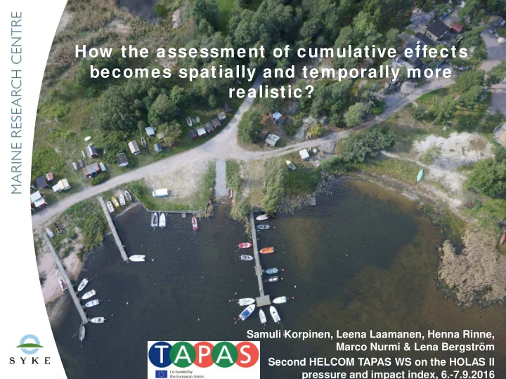
How the assessment of cumulative effects becomes spatially and temporally more realistic?

Samuli Korpinen, Leena Laamanen, Henna Rinne, Marco Nurmi & Lena Bergström Second HELCOM TAPAS WS on the HOLAS II pressure and impact index, 6.-7.9.2016

Impact chains from activities to pressures and impacts

Sectors and human activities Pressures Impacts on specific habitats and species

Lost seabed habitat (km2): Cumulative sum over the assessment

• period. Spatial overlaps avoided.

How to make the aggregated pressure layers?

Hunted/killed animals (individuals): Average of the annual number between the assessment years. All species summed/ averaged? Fish catch (tons): Average of the annual number between the assessment years. All species summed. Physical disturbance (several metrics): Average of the annual number between the assessment years. All species summed/ averaged? Inputs (tons): Average of the annual number between the assessment years. All nutrients summed.

3

Physical disturbance

How to aggregate pressures of different metrics?

Biological disturbance Inputs of contaminants Bottom-trawling fishery Disposal of dredged matter Sand extraction Shipping Capital dredging

Pressure magnitude

Category Human activity Weight >80-100% Bottom-trawling fishery Capital dredging 1 >60-80% Disposal of dredged matter Sand extraction 0.8 >40-60% 0.6 >20-40% Shipping 0.4 >0-20% 0.2

4

Spatial ’buffer’ around the points/lines/polygons:

• Initial scores by the TAPAS project team
• BalticBOOST literature review
• TAPAS expert survey

How to apply the pressure gradients to the data layers?

Riverine pollution:

• Satellites images from spring-time turbidity is used as the

proxy for inputs of nutrients, contaminants and possibly

• ther substances such as suspended solids or organic

matter.

5

Attenuation of pressures from their source

Two sources of information:

• Expert survey
• BalticBOOST literature review

Type A Type B Type C Type D

Riverine gradients taken directly from the satellite images.

6

Energy affects the pressure intensity

Physical disturbance Input of nutrients Input of contaminants Input of beach litter Input of org. matter Input of heat

7

Which pressures attenuate towards deeper waters?

Water depth suppresses some pressures

Input of heat Disturbance of species due to human presence Changes to hydrological conditions Which curves could describe that?

Type A Type B Type C Type D

Shipping: physical disturbance

8

Pressures accumulating over years

How to consider different temporal frequency

• f pressures in the data layers?

Pressures taking place less frequently Seasonality of the pressures and ecosystem components Input of litter Physical loss Introductions of NIS

• All others. E.g. nutrient inputs are taken up by the primary

production, fish stocks reproduce, sediment disturbance settles, etc.

9

10