Hoare logic and Model checking If we can express the artefact as a - PowerPoint PPT Presentation

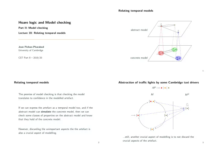
Hoare logic and Model checking If we can express the artefact as a temporal model too, and if the crucial aspects of the artefact. ...still, another crucial aspect of modelling is to not discard the M Abstraction of traffjc lights by some Cambridge taxi drivers 2 also a crucial aspect of modelling. However, discarding the unimportant aspects the the artefact is Part II: Model checking check some classes of properties on the abstract model and know abstract model can simulate the concrete model, then we can that they hold of the concrete model. translates to confjdence in the modelled artefact. CST Part II – 2019/20 Lecture 10: Relating temporal models Jean Pichon-Pharabod University of Cambridge The premise of model checking is that checking the model 3 Relating temporal models concrete model abstract model 1 Relating temporal models AP ::= • | • | • M # {• , •} {•} {•} {•} {•}

Temporal model simulation 1/2 5 s 1 0 R s 0 s 1 0 1 R R Examples of simulations 1 The identity relation is a simulation: The terrible punter (lecture 1) can simulate the good punter (lecture 3) by, when it has a choice of things, doing a good thing. 6 Examples of simulations . . . M R s 0 7 (1) R is consistent with labels: (continued on the next slide) 4 Temporal model simulation 2/2 R -related start state to some R -related end state: R is a temporal model simulation of M by M ′ : (3) any step in M can be matched by a step in M ′ from any ➀ � ➂ ➁ ∈ ( M ∈ TModel ) → ( M ′ ∈ TModel ) → ( M � S → M ′ � S → Prop ) → Prop   ∀ s 0 , s 1 ∈ M � S , s ′ 0 ∈ M ′ � S . M � R M ′ def = s 0 M � T s 1 ∧ s 0 R s ′ 0 →      ∃ s ′ 1 ∈ M ′ � S .    s ′ 0 M ′ � T s ′ 1 ∧ s 1 R s ′ ∀ s ∈ M . S , s ′ ∈ M ′ � S . � � ∧ s R s ′ → ∀ p ∈ AP . M ′ � ℓ s ′ p → M � ℓ s p s ′ s ′ (2) R relates initial states of M to initial states in M ′ : → ∃ s ′ 1 . ( ∀ s ∈ M � S . M � S 0 s → ∃ s ′ ∈ M ′ � S . M ′ � S 0 s ′ ∧ s R s ′ ) ∧ M ′ � T M � T M � T s ′ M ′ { even } ∀ M ∈ TModel . { odd } { even } let R = ( s �→ s ) in M � R M { even } { odd } { odd } { even } { odd }

Milner’s tea & cofgee machines Often, the details of the simulation are not so important, what def important, often what matters is the existence of a bisimulation: As for simulations, the details of the bisimulation are not so Temporal model bisimulation 10 very fragile, and really depends on left-totality! to know it holds of the more concrete model. It suffjces to show the property holds of the more abstract model compatible with the simulation preorder: possibly fewer states and transitions. behaviour, making it less precise, but that allows it to have def matters is the existence of a simulation: 9 Temporal model simulation M nice 8 11 M bad ∅ ∅ ➀ � ➁ ∈ TModel → TModel → Prop ( M � M ′ ) = ∃ R . M � R M ′ { £ } { £ } { £ } It means that M ′ is “more abstract” than M : it may have more { } { } { � } { � } Simulation preserves ACTL ∗ R is a temporal model bisimulation of M by M ′ : The universal, implication-free fragment of CTL ∗ , ACTL ∗ IF , is ➀ ≈ ➂ ➁ ∈ ( M ∈ TModel ) → ( M ′ ∈ TModel ) → ∀ M ∈ TModel , M ′ ∈ TModel , ψ ∈ StateProp ( M � S → M ′ � S → Prop ) → Prop ACTL ∗ IF . = M � R M ′ ∧ M ′ � R M ( M � M ′ ∧ us ψ ∧ M ′ � ψ ) → M � ψ M ≈ R M ′ def ➀ ≈ ➁ ∈ TModel → TModel → Prop This property can seem strange, because F φ has an existential feel to it. In fact, it is ( M ≈ M ′ ) = ∃ R . M ≈ R M ′

15 This is the approach taken by TLA+. with one step of the abstract model? number of times in any state (in addition to allowing forever on states with self-loops). We can then adapt most of the notions we have seen so far. However, in this setting, we do not want to use the X temporal operator. 14 Revisiting stuttering Summary We saw how abstraction can be used to relate temporal models in a way that makes checking some classes of properties sound. ...but remember an important part of modelling is judicious In the next lecture, we will look at how to implement model checking. What if we want to abstract multiple steps of the concrete model 13 For example, on a variation of the tea & cofgee machines example: � but in general not the other way around! 12 Bisimulation and simulations Bisimulation implies simulations in both directions Bisimulation preserves CTL ∗ M ≈ M ′ → ( M � M ′ ∧ M ′ � M ) All of CTL ∗ is compatible with bisimulation equivalence: ∀ M ∈ TModel , M ′ ∈ TModel , ψ ∈ StateProp WI . ∅ ∅ M ≈ M ′ → ( M � ψ ↔ M ′ � ψ ) { £ } { £ } { £ } { } { } � We can change our notion of path to allow staying any fjnite under-approximation! � domain knowledge is crucial.