SLIDE 1
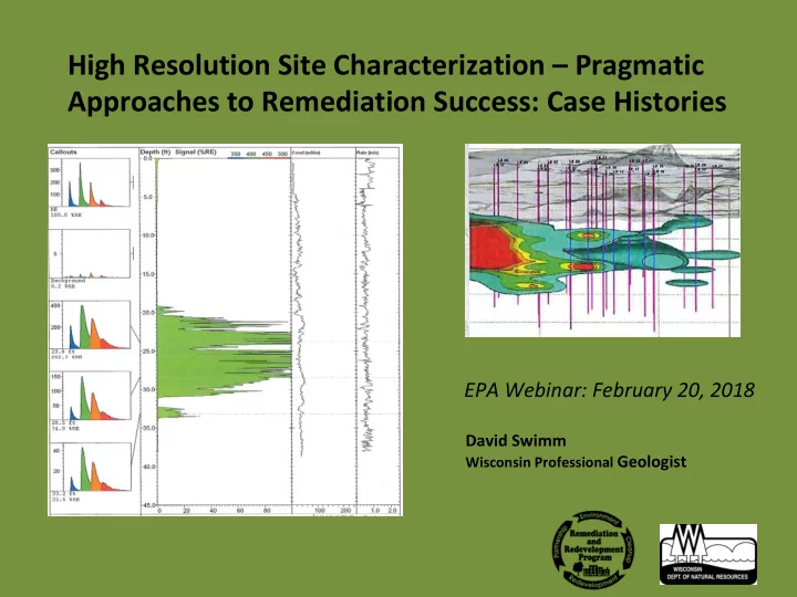
High Resolution Site Characterization – Pragmatic Approaches to Remediation Success: Case Histories
David Swimm
Wisconsin Professional Geologist
EPA Webinar: February 20, 2018
SLIDE 2 Site 2:
- Confirmed post-remedy shallow LNAPL distribution
- Indicated lack of any deeper LNAPL accumulation
- Provided detailed soil distributions
- Denied funding for further active treatment
- Helped focus additional work – confirmation potable well sampling
and vapor intrusion (VI) assessments
Two LNAPL Remedial Case Histories:
- Both had expensive, historical remedies performed
- Both had relatively poor results
- Both had post-remedy, high resolution surveys conducted (LIF/EC)
that resulted in the following: Site 1 :
- Provided improved focus on LNAPL distribution
- Provided context (soil distributions) for LNAPL accumulations
- Approved funding for a second remedial action
SLIDE 3 Site 1 - Post-Remedy Perceived LNAPL Distribution
Subject Site
system
- Operated 2003-07
- Extracted diesel and
gasoline (two sources)
- 7K gals. LNAPL reportedly
removed
- $670K reimbursed
- MWs still contain 2-4 ft.
LNAPL post-remedy
impacted post-remedy
Station Bldg.
LNAPL Accumulation
Additional LUST Sites w/LNAPL
SLIDE 4
Post-Remedial LNAPL Lateral Distribution
SZ SM SW SP SP SP
Top Elevated PID
1997 Investigation Section
SLIDE 5 LNAPL Signal:
- Laser provided UV light induces some LNAPL compounds to excite enough to
emit light (fluorescence) that reflects back to tool
- Fluorescence response is calibrated to a known LNAPL standard - plotted as a
percentage of Reference Emitter (%RE)
- Frequency spectrum (i.e., “waveform callouts”) of induced fluorescence can
differentiate product types
- Low range responses can include false positives
Soil Discriminator - Electrical Conductivity (EC):
- Conductivity between dipoles
- Lower EC reflects coarse grained soils; higher reflects finer grained soils,
including clay minerals which can enhance electrical flow
Conducted Laser Induced Fluorescence (LIF) Survey during 2012
Performed LNAPL Transmissivity (Tn)Testing:
- Results were 0.15 - 0.40 ft2/d
- Eliminated further consideration of hydraulic removals
SLIDE 6
26.5 24.8
MW-3 50% RE 10% RE
Example LIF Boring Log: LIF-9 Located near MW-3
SM
RE= Reference Emitter
ML & SM Electrical Conductivity Penetration Rate Waveform Callouts 30 mS/m SW
Fluorescence Signal
SLIDE 7
Net Feet >10%RE Signal
(Smear Zone at 17-26’ bgs)
0.5 1.9 0.9 2.1 2.3 2.8 1.7 2.8
G Diesel LNAPL plume Gasoline LNAPL plume
0.5
>1.0 net feet
1 .
NA
LIF boring (contoured values) Well LNAPL Thickness (red) upper smear zone signal
L10 L12 L9
SLIDE 8
5050%%“More Focused”
Net Feet >50% RE Signal
(Smear Zone at 17-26’ bgs)
SLIDE 9
Net Feet >10%RE Signal
(Below Smear Zone: > 26’bgs)
L9
SLIDE 10
Improved Lateral LNAPL Resolution Old New
SLIDE 11
SM SW GW/SW
Soil Sieve Analyses
LIF Boring EC Responses w/Sieve Results
Soil Type Distribution - Smear Zone Interval
A A’ B B’ 1997 Boring Log X-Section L12 L10
SLIDE 12
SZ L 19 L 9 L 12 L 13 L 16 L 17 L 18 16 20 24 28 32 36 40 S X SZ
A A’
SM SW
LIF > 50% RE LIF 10-50% RE 20 ft.
(approx. horizontal scale)
GW/SW
Soil Type Distribution - Smear Zone Interval
LIF Boring EC Responses
SLIDE 13
SP SP SW SZ
SM
SZ
LIF-Indicated LNAPL
SW SM SM
Old New
Improved Vertical LNAPL Resolution & Geologic Context
PID suggested LNAPL smear zone
SLIDE 14 LIF Survey results need to be interpreted and integrated:
- They are expensive
- Fluorescence results provide formation LNAPL thickness
independent of wells, and can distinguish between product types
- Conductivity results provide detailed smear zone soil
distributions in much greater detail than boring logs
- Integrated results provide LNAPL distributions within their
geologic context, including accumulations below the water table
Lessons Learned
LIF Survey & LNAPL Transmissivity (Tn) Results SVE Pilot Testing
SLIDE 15
Smear Zone SVE Pilot Test Results
(Inches of Water Column) SM 60 ft.
10 1 0.5 27 66 1
SM 60 ft. Pilot Test Extraction Well Site 1 EC-based soil transition Site 1
SLIDE 16 SVE Operation - Gasoline Sources:
- 2 year operation (10/15 - present)
- Single system w/extraction from
both sites
- 8,500 gals. LNAPL extracted to-
date (9/17)
- Anticipate 10,000+ gals. by shut-
down Excavation – Diesel Source:
- Approx. 2,500 tons removed
- Included some mass below water
table
Remedial Results
Bldg.
SM
Diesel Source Excavation SVE Extraction Well System Bldg.
SLIDE 17 Remedies conducted:
- Limited Excavations
- DPE Extraction – 5 wells
Credible operations 2009-12 3K gallons LNAPL removed
- $600K reimbursed (overall)
Risks Still Present:
including confined
- Potable well risk
- PVI risk
Consultant requested additional funds for system re-start and expansion
Site 2 Post-System, 2013 LIF Boring Survey
Excavation Areas Recovery Well Drinking Water Wells LIF Borings
SLIDE 18 LIF Response (%RE)
Maximum Amplitude Map Problems:
LNAPL formation thickness
- Does not show soil/geology
context for accumulation
confined accumulation
LIF 3 LIF 16 LIF 15
SLIDE 19
LIF-15 LIF-16
Amplitude “Bulls Eye”
(Water Table LNAPL Accumulation)
Maximum Fluorescence Responses
SLIDE 20 Recon: “Meaningful” LNAPL Signal
(Confined LNAPL Beneath Roadway)
Fluorescence Bias (25% RE) EC Response – Soil Discriminator Finer Grained Soils →
LIF Bias - discriminates robust signal:
- Likely >LNAPL sats.
- Eliminates noise
- Look to correlate w/
well accumulations Again, max response does not discriminate LNAPL thickness Base confinement
LIF-3
OW-7
(nearby/contains LNAPL)
SLIDE 21
smear zone Conductivity Bias (~70 mS/m) Sieve Calibration: ML (64% fines) Correlation Markers (3)
Base 1st Confining Top 2nd Confining
ML
SM
LIF-3
25% RE
Soil Interpretation
SLIDE 22 * * * * *
Previous Slide Slide 19 1
s t
C
f i n i n g L a y e r 2nd Confining Layer OW-2 LIF-15 LIF-14
Confirmed LNAPL Accumulation
Well & borings that intersect confined LNAPL
SLIDE 23
? ? ?
Consultant Indicated Residual LNAPL Volume
LIF 16 ? ?
Slide 25
SLIDE 24
Conductivity Bias (~70 mS/m)
Fluorescence Bias (25% RE)
Base 1st Confining Top 2nd Confining
ML SM
LIF-16
no response
SLIDE 25 40’
Bldg.
Predominant Soils – Beneath 1st Confining
(EC-based Interpretation)
LIF Borings Regional GW Flow ML ML SM SW
- Explained local, lateral flow
deviation from regional
wells to the NW
sampled potable wells (clean) were too close
Confined LNAPL
(defined by LIF 3 & well/borings)
Site 2: Improved GW Flow Interpretation:
X X X
SLIDE 26 Did not approve funding for renewed DPE treatment or system expansion NA assessment showed significant post-treatment reductions, especially along the upper (water table) portion
By elimination helped us focus on remaining risk pathways:
- Expanded potable well sampling - NW and downgradient
- VI risk, not related to the LIF-defined LNAPL
Site 2 Interpreted LIF Survey Results - Practical Implications