High Dimensional Data PCA So far we ve considered scalar data - PDF document

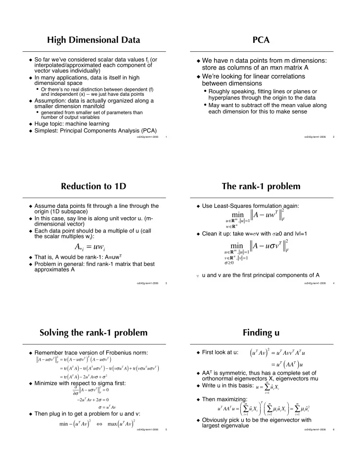
High Dimensional Data PCA � So far we � ve considered scalar data values f i (or � We have n data points from m dimensions: interpolated/approximated each component of store as columns of an mxn matrix A vector values individually) � We � re looking for linear correlations � In many applications, data is itself in high dimensional space between dimensions • Or there � s no real distinction between dependent (f) • Roughly speaking, fitting lines or planes or and independent (x) -- we just have data points hyperplanes through the origin to the data � Assumption: data is actually organized along a • May want to subtract off the mean value along smaller dimension manifold each dimension for this to make sense • generated from smaller set of parameters than number of output variables � Huge topic: machine learning � Simplest: Principal Components Analysis (PCA) cs542g-term1-2006 1 cs542g-term1-2006 2 Reduction to 1D The rank-1 problem � Assume data points fit through a line through the � Use Least-Squares formulation again: 2 origin (1D subspace) A � uw T min � In this case, say line is along unit vector u. (m- u � R m , u = 1 F dimensional vector) w � R n � Each data point should be a multiple of u (call � Clean it up: take w= � v with � � 0 and |v|=1 the scalar multiples w i ): 2 A * i = uw i A � u � v T min u � R m , u = 1 F � That is, A would be rank-1: A=uw T v � R n , v = 1 � � 0 � Problem in general: find rank-1 matrix that best approximates A � u and v are the first principal components of A cs542g-term1-2006 3 cs542g-term1-2006 4 Solving the rank-1 problem Finding u 2 = u T Avv T A T u ( ) u T Av � First look at u: � Remember trace version of Frobenius norm: 2 = tr A � u � v T ( ) ( ) T A � u � v T A � u � v T ( ) u = u T AA T F ( ) � tr A T u � v T ( ) � tr v � u T A ( ) + tr v � u T u � v T ( ) = tr A T A � AA T is symmetric, thus has a complete set of ( ) � 2 u T Av � + � 2 = tr A T A orthonormal eigenvectors X, eigenvectors mu � Minimize with respect to sigma first: m � � Write u in this basis: � 2 = 0 u = ˆ u i X i � � A � u � v T i = 1 F � 2 u T Av + 2 � = 0 � Then maximizing: T � � � � m m m � = u T Av � � � u T AA T u = µ i ˆ � = µ i ˆ ˆ 2 u i X i u i X i u i � � � � � � � � Then plug in to get a problem for u and v: i = 1 i = 1 i = 1 ( ) ( ) � Obviously pick u to be the eigenvector with min � u T Av max u T Av 2 2 � largest eigenvalue cs542g-term1-2006 5 cs542g-term1-2006 6

Finding v Generalizing � Write the thing we � re maximizing as: � In general, if we expect problem to have 2 = v T A T uu T Av ( ) subspace dimension k, we want the u T Av closest rank-k matrix to A ( ) v = v T A T A • That is, express the data points as linear combinations of a set of k basis vectors � Same argument gives v the eigenvector (plus error) corresponding to max eigenvalue of A T A • We want the optimal set of basis vectors and the optimal linear combinations: � Note we also have 2 = max � AA T 2 � 2 = u T Av ( ) ( ) = max � A T A ( ) = A 2 A � UW T min 2 U � R m � k , U T U = I F W � R n � k cs542g-term1-2006 7 cs542g-term1-2006 8 Finding W Finding U � Plugging in W=A T U we get � Take the same approach as before: 2 = tr A � UW T ( ) ( ) T A � UW T A � UW T 2 min A � UW T F F = tr A T A � 2tr WU T A + tr WU T UW T � min � 2tr A T UU T A + tr A T UU T A 2 � 2tr WU T A + W � max tr U T AA T U = A F 2 F � Set gradient w.r.t. W equal to zero: � AA T is symmetric, hence has a complete set of orthogonormal eigenvectors, say � 2 A T U + 2 W = 0 columns of X, and eigenvalues along the diagonal of M (sorted in decreasing order): W = A T U AA T = XMX T cs542g-term1-2006 9 cs542g-term1-2006 10 Finding U cont’d Back to W � Our problem is now: � We can write W=V � T for an orthogonal V, and maxtr U T XMX T U square kxk � � Note X and U are both orthogonal, so is X T U, � Same argument as for U gives that V should be Z T Z = I tr Z T MZ which we can call Z: the first k eigenvectors of A T A max � What is � ? k m � � � From earlier rank-1 case we know � max µ j Z ji 2 � 11 = � = A 2 = A T Z T Z = I i = 1 j = 1 2 � Since U *1 and V *1 are unit vectors that achieve � Simplest solution: set Z=( I 0) T which means that the 2-norm of A T and A, we can derive that first U is the first k columns of X row and column of � is zero except for diagonal. (first k eigenvectors of AA T ) cs542g-term1-2006 11 cs542g-term1-2006 12

What is � The Singular Value Decomposition T from A � Going all the way to k=m (or n) we get the � Subtract rank-1 matrix U *1 � 11 V *1 Singular Value Decomposition (SVD) of A • zeros matching eigenvalue of A T A or AA T � A=U � V T � Then we can understand the next part of � � The diagonal entries of � are called the singular values � End up with � a diagonal matrix, � The columns of U (eigenvectors of AA T ) are the containing the squareroots of the first k left singular vectors eigenvalues of AA T or A T A (they � re equal) � The columns of V (eigenvectors of A T A) are the right singular vectors � Gives a formula for A as a sum of rank-1 � matrices: A = � i u i v i T i cs542g-term1-2006 13 cs542g-term1-2006 14 Cool things about the SVD Least Squares with SVD A 2 = � 1 � 2-norm: � Define pseudo-inverse for a general A: 2 = � 1 2 + � + � n 2 A F � Frobenius norm: T A + = V � + U T = n v i u i � � Rank(A)= # nonzero singular values � i • Can make a sensible numerical estimate i = 1 � Null(A) spanned by columns of U for zero � i > 0 singular values � Note if A T A is invertible, A + =(A T A) -1 A T � Range(A) spanned by columns of V for nonzero • I.e. solves the least squares problem] singular values A � 1 = V � � 1 U T � For invertible A: � If A T A is singular, pseudo-inverse defined: A + b is the x that minimizes ||b-Ax|| 2 and of n T v i u i � = all those that do so, has smallest ||x|| 2 � i i = 1 cs542g-term1-2006 15 cs542g-term1-2006 16 Solving Eigenproblems The Symmetric Eigenproblem � Computing the SVD is another matter! � Assume A is symmetric and real � We can get U and V by solving the symmetric � Find orthogonal matrix V and diagonal matrix D eigenproblem for AA T or A T A, but more s.t. AV=VD specialized methods are more accurate • Diagonal entries of D are the eigenvalues, corresponding columns of V are the eigenvectors � The unsymmetric eigenproblem is another � Also put: A=VDV T or V T AV=D related computation, with complications: • May involve complex numbers even if A is real � There are a few strategies • If A is not normal (AA T � A T A), it doesn � t have a full • More if you only care about a few eigenpairs, not the basis of eigenvectors complete set… • Eigenvectors may not be orthogonal… Schur decomp � Also: finding eigenvalues of an nxn matrix is � Generalized problem: Ax= � Bx equivalent to solving a degree n polynomial • No “analytic” solution in general for n � 5 � LAPACK provides routines for all these • Thus general algorithms are iterative � We � ll examine symmetric problem in more detail cs542g-term1-2006 17 cs542g-term1-2006 18