Network Calculus: Reference Material: J.-Y. LeBoudec and Patrick - - PDF document

CPSC-663: Real-Time Systems Network Calculus 1

Network Calculus:

• Reference Material:

J.-Y. LeBoudec and Patrick Thiran: “Network Calculus: A Theory of Deterministic Queuing Systems for the Internet”, Springer Verlag Lecture Notes in Computer Science No. 2050.

• Network Calculus as system theory for computer networks.
• Some mathematical background
• Arrival Curves
• Service Curves
• Network Calculus Basics

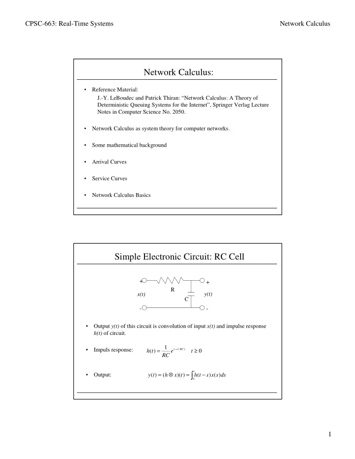
Simple Electronic Circuit: RC Cell

• Output y(t) of this circuit is convolution of input x(t) and impulse response

h(t) of circuit.

• Impuls response:
• Output:

+

• +
• x(t)

y(t) R C 1 ) (

) / (

≥ =

−

t e RC t h

RC t

∫

− = ⊗ =

t

ds s x s t h t x h t y ) ( ) ( ) )( ( ) (

CPSC-663: Real-Time Systems Network Calculus 2

Greedy Shaper

• A shaper forces an input traffic flow x(t) to have an output y(t) which adheres

to an envelope σ.

• The output function y(t) can be derived as follows:
• Other analogies apply as well (commutativity and associativity), which allow

to extend this analysis to large-scale systems.

• There are significant differences, though!

)} ( ) ( { inf ) )( ( ) ( s x s t t x t y

t s

+ − = ⊗ =

≤ ≤

σ σ

Min-Plus Calculus: Infimum vs. Minimum

• Let S be nonempty subset of R.

Definition [Infimum] inf(S) = (M s.t. s ≥ M ∀ s ∈ S) inf(ø) = +∞ Definition [Minimum] min(S) = ( M ∈ S s.t. s ≥ M ∀ s ∈ S)

• Notation: ^ denotes infimum (e.g. a ^ b = min{a,b})

CPSC-663: Real-Time Systems Network Calculus 3

The Dioid (R ∪ {+∞}, ^, +)

• Conventional (“plus-times”) algebra operates on algebraic structure (R,+,*).
• Min-plus algebra replaces operations:

– “addition” becomes “computation of infimum” – “multiplication” becomes “addition”

• Resulting algebraic structure becomes (R ∪ {+∞}, ^, +)
• Example:

– Conventional algebra: (3+4) * 5 = (3*5) + (4*5) = 15 + 20 – min-plus algebra: (3^4) + 5 = (3 + 5) ^ (4 + 5) = 8 ^ 9 = 8

• (Closure of ^) For all a,b ∈ R ∪ {+∞}, a ^ b ∈ R ∪ {+∞}
• (Associativity of ^) For all a,b,c ∈ R ∪ {+∞}, (a^b)^c=a^(b^c)
• (Existence of a zero element of ^) There is some e ∈ R ∪ {+∞}, such that

for all a ∈ R ∪ {+∞}, a ^ e = a.

• (Idempotency of ^) For all a ∈ R ∪ {+∞}, a ^ a = a.
• (Commutativity of ^) For all a,b ∈ R ∪ {+∞}, a ^ b = b ^ a.
• (Closure of +) For all a,b ∈ R ∪ {+∞}, a + b ∈ R ∪ {+∞}.
• (Zero element of ^ is absorbing for +) For all a ∈ R ∪ {+∞},

a + e = e = e + a.

• (Existence of neutral element for +) There is some u ∈ R ∪ {+∞} such

that for all a ∈ R ∪ {+∞}, a + u = a = u + a.

• (Distributivity of + with respect to ^) For all a,b,c ∈ R ∪ {+∞},

(a ^ b) + c = (a + c) ^ (b + c) = c + (a ^ b)

Properties of (R ∪ {+∞}, ^, +)

CPSC-663: Real-Time Systems Network Calculus 4

Wide-Sense Increasing Functions

Definition [wide-sense increasing] A function is wide-sense increasing iff f(s) ≤ f(t) for all s ≤ t.

• Define G as the set of non-negative wide-sense increasing functions.
• Define F as the set of non-negative wide-sense increasing functions with

f(t) = 0 for t < 0.

• Operations on functions:

(f + g)(t) = f(t) + g(t) (f ^ g)(t) = f(t) ^ g(t)

Wide-Sense Increasing Functions

• Peak rate function λR:

“Rate” R

• Burst delay function δT:

“Delay” T

R

   > =

• therwise

if ) ( t Rt t

R

λ

T

   > ∞ + =

• therwise

if ) ( T t t

T

δ

CPSC-663: Real-Time Systems Network Calculus 5

Wide-Sense Increasing Functions (2)

• Rate latency function βR,T:

“Rate” R , “Delay” T

• Affine functions γr,b:

“Rate” r, “Burst” b

R

   > − =

• therwise

if ) ( ) (

,

T t T t R t

T R

β    > + =

• therwise

if ) (

,

t b rt t

b r

γ

T

r

b

Wide-Sense Increasing Functions (3)

• Step function υT:
• Staircase function uT,τ:

“Interval” T, “Tolerance” τ    > =

• therwise

if 1 ) ( T t t

T

υ      >       + =

• therwise

if ) (

,

t T t t uT τ

τ

T

1 1 2 3

τ

T

CPSC-663: Real-Time Systems Network Calculus 6

Wide-Sense Increasing Functions (4)

• More general functions in F can be constructed by combining basic

functions.

• Example 1: r1>r2>...>rI and b1<b2<...<bI
• Example 2:

RT 2RT 3RT

{ }

i i I I

b r I i b r b r b r

f

, 1 , , , 1

min

2 2 1 1

γ γ γ γ

≤ ≤

= ∧ ∧ ∧ = K

r1 r2 r3 b1 b2 b3

T 2T 3T 4T 5T

{ }

iRT RT RT f

iT R i T R T R R

+ = ∧ + ∧ + ∧ =

≥ 2 , 4 , 2 , 2

inf } 2 { } { β β β λ K

Pseudo-Inverse of Wide-Sense Increasing Functions

Definition [Pseudo-inverse] Let f be a function of F. The pseudo-inverse of f is the function f-1(x) = inf{t such that f(t) ≥ x}.

• Examples:

λR

• 1

= λ1/R δT

• 1

= δ0 ^ T βR,T

• 1

= γ1/R,T γr,b

• 1

= β1/r,b

CPSC-663: Real-Time Systems Network Calculus 7

Properties of Pseudo-Inverse

• (Closure)
• (Pseudo-inversion) We have that
• (Equivalent definition)

x t f t x f t x f x t f ≥ ⇒ < ≤ ⇒ ≥

− −

) ( ) ( ) ( ) (

1 1

} ) ( such that sup{ ) (

1

x t f t x f < =

−

) ( and

1 1

= ∈

− −

f F f

Min-Plus Convolution

• Integral of function f(t) ( f(t) = 0 for t ≤ 0 ) in conventional algebra:
• “Integral” for same function f(t) in min-plus algebra:
• Convolution of two functions f(t) and g(t) that are zero for t < 0 in

conventional algebra: Definition [Min-plus convolution] Let f and g be two functions of F. The min-plus convolution of f and g is the function

∫

t

ds s f ) (

{ }

) ( inf

such that

s f

t s s ≤ ≤ ℜ ∈

( )

∫

+ − = ⊗

t

ds s g s t f t g f ) ( ) ( ) (

{ }

) ( ) ( inf ) )( ( s g s t f t g f

t s

+ − = ⊗

≤ ≤

CPSC-663: Real-Time Systems Network Calculus 8

Min-Plus Convolution: Example 1

• Compute (γr,b⊗ βR,T)(t)
• Case 1: 0 ≤ t ≤ T

Case 2: t > T

{ } { }

) ( ) ( inf ) ( ) ( inf ) )( (

, , , , , ,

= + = + − = + − = ⊗

≤ ≤ ≤ ≤ b r b r t s T R b r t s T R b r

s t s s t t γ γ β γ β γ

{ } { } { } { }

{ } { } { }

{ }

)} ( { )} ( { )} ( { )} ( { )} ( { )} ( { ) ( inf )} ( { )} ( { ) ( ) ( inf ) ( inf ) ( ) ( inf ) ( ) ( inf ) ( ) ( inf ) ( ) ( inf ) )( (

, , , , , , , , , ,

T t R T t r b T t R T t r b T t r b T t R s r R RT rt b T t r b T t R T s R s t r b s t r b s s t s s t s s t s s t t

t s T t s T T s T R b r t s T R b r t s T T R b r T s T R b r t s T R b r

− ∧ − + = − ∧ − + ∧ − + = − ∧ − + − + ∧ − + = − + ∧ − + − + ∧ + − + = + − ∧ + − ∧ + − = + − = ⊗

≤ ≤ ≤ ≤ ≤ ≤ = ≤ ≤ ≤ ≤ ≤ ≤

β γ β γ β γ β γ β γ

Min-Plus Convolution: Example 1 (2)

(γr,b⊗ βR,T)(t)

r R T b

CPSC-663: Real-Time Systems Network Calculus 9

Min-Plus Convolution: Example 2

δT ⊗ λR = ?

{ } { } { }

) ( inf ) ( ) ( inf ) )( ( : ) ( 1 Case ) ( ) ( inf ) )( ( = + = + − = ⊗ ≤ ≤ + − = ⊗

≤ ≤ ≤ ≤ ≤ ≤

s s s t t T t s s t t

R t s R T t s R T R T t s R T

λ λ δ λ δ λ δ λ δ

{ } { } { } { }

T R R R t s T R T s T R t s T T R T s T R R T

T t s t s t s s t s s t t t T t

,

) ( ) ( inf ) ( inf ) ( ) ( inf ) ( ) ( inf ) )( ( ) )( ( : ) ( 2 Case β λ λ λ δ λ δ λ δ λ λ δ = − = ∞ + − ∧ + − = + − ∧ + − = ⊗ = ⊗ >

≤ < ≤ ≤ ≤ < ≤ ≤

Models for Data Flow

• Consider system S: receives input data, and delivers data after a variable

delay.

• R(t) is cumulative input function at time t.
• R*(t) is cumulative output function at time t.

Definition [Backlog] The backlog at time t is R(t)-R*(t). Definition [Virtual Delay] The virtual delay at time t is d(t) = inf{τ ≥ 0 : R(t) ≤ R*(t + τ)} S R(t) R*(t)

CPSC-663: Real-Time Systems Network Calculus 10

Virtual Delay

d(t) = inf{τ ≥ 0 : R(t) ≤ R*(t + τ)}

• If input and output are continuous

R*(t + d(t)) = R(t) (*) d(t) is smallest value satisfying (*)

R*(t) R(t)

t1 t2

Arrival Curves

Definition [Arrival Curve α(.) α(.) α(.) α(.)] Given a wide-sense increasing function α(.) defined for t ≥ 0 (i.e. α(.) ∈ F) we say that a flow R is constrained by α(.) iff for all s ≤ t: R(t) – R(s) ≤ α(t – s).

• “R has α(.) as arrival curve.”
• “R is bounded by α(.).”
• “R is α-smooth.”
• Note:

– α(.) is in the interval-domain. – for all s ≥ 0 and I ≥ 0, R(s + I) – R(s) ≤ α(I).

CPSC-663: Real-Time Systems Network Calculus 11

Arrival Curves (2)

α(t)

time

bits

time t bits

Example: Affine Arrival Curve γr,b

• α(t) = rt

Flow is peak-rate limited. For example when physical bit rate is limited.

• α(t) = b

Maximum number of bits ever sent is at most b.

• α(t) = rt + b Leaky bucket with rate r and burst tolerance b.
• A leaky bucket constrains the arrival to the affine arrival curve γr,b = rt + b.

CPSC-663: Real-Time Systems Network Calculus 12

Example: Staircase Function uT,τ

Definition [Generic Cell Rate Algorithm GCRA(T,τ τ τ τ)] The Generic Cell Rate Algorithm (GCRA) with parameters (T,τ) is used with fixed size packets, called cells and defines conformant cells as follows: It takes as input a cell arrival time t and returns result. It has an internal (static) variable tat (theoretical arrival time). – initially, tat = 0 – when a cell arrives at time t, then

if (t < tat – tau) result = NON-CONFORMANT else { tat = max(t, tat) + T; result = CONFORMANT; }

• For cells of size k, GCRA(T,τ) constrains flows to the staircase arrival

function k uT,τ(.).

Equivalence of Leaky Bucket and GCRA

For a flow with packets of constant size δ, satisfying the GCRA(T,τ) is equivalent to satisfying a leaky bucket controller with rate r and burst tolerance b given by: b = (τ/T + 1) δ and r = δ / T Applications to ATM and Intserv:

• Constant Bit Rate (CBR) in ATM:

– Single GCRA controller with parameters T (ideal cell interval) and τ (cell delay variation tolerance).

• Variable Bit Rate (VBR) in ATM:

– Two GCRA controllers.

• Intserv: T-SPEC (p,M,r,b) with peak rate p, maximum packet size M,

sustainable rate r, and burst tolerance b. α(t) = min(M + pt, rt + b)

CPSC-663: Real-Time Systems Network Calculus 13

Sub-Additivity

Definition [Sub-additive function] Let f be a function of F. Then f is sub-additive iff f(t + s) ≤ f(t) + f(s) for all s, t ≥ 0 .

• Notes:

– If f(0) = 0, this is equivalent to imposing that f = f ⊗ f . – Concave functions passing through origin are sub-additive. – While concavity and convexity are simple to check visually, sub- additivity is not.

R RT T

βR,T(t)+K’

K’ R RT T

βR,T(t)+K’’

K’’

Sub-Additive Closure

Definition [Sub-additive closure] Let f be a function of F. Denote f(n) the function obtained by repeating (n-1) convolutions of f with itself. By convention, f(0)=δ0, so that f(1) = f, f(2) = f ⊗f, etc. Then the sub-additive closure of f, denoted by f∞, is defined by f∞ = δ0 ^ f ^ (f ⊗f) ^ (f ⊗f ⊗f) ^ ... = infn≥0{f(n)}

• The sub-additive closure is the largest sub-additive function smaller than f

and zero in t = 0.

CPSC-663: Real-Time Systems Network Calculus 14

Sub-Additive Closure: Example

R RT T

βR,T(t)+K’

K’ R RT T

βR,T(t)+K’=(βR,T(t)+K’) ∞

K’ R RT T

βR,T(t)+K’’

K’’ T K’’

(βR,T(t)+K’’) ∞

2T 3T 4T 5T 2K’’ 3K’’ 4K’’

Sub-Additivity and Arrival Curves

Theorem: [Reduction of Arrival Curve to a Sub-Additive One] Saying that a flow is constrained by a wide-sense increasing funtion α(.) is equivalent to saying that it is constrained by the sub-additive closure α∞(.). Lemma: A flow R is constrained by arrival curve α iff R ≤ R ⊗ α. Lemma: If α1 and α2 are arrival curves for a flow R, then so is α1 ⊗ α2.

CPSC-663: Real-Time Systems Network Calculus 15

Min-Plus Deconvolution and Traffic Envelopes

Definition [Min-Plus Deconvolution] Let f and g be two functions of F. The min-plus deconvolution of f by g is the function (f ∅ g)(t) = supu≥0{f(t + u) – g(u)}. Definition [Minimum Arrival Curve – or Envelope] The envelope of a flow R is defined by R ∅ R. By definition, we have (R ∅ R)(t) = supv≥0{R(t + v) – R(v)}.

Envelopes: Examples

( Figures from J.-Y. LeBoudec and Patrick Thiran: “Network Calculus: A Theory of Deterministic Queuing Systems for the Internet”, Springer Verlag Lecture Notes in Computer Science )

CPSC-663: Real-Time Systems Network Calculus 16

Service Curves

Example 1: Generalized Processor Sharing (GPS)

• During any busy period (flow is backlogged) of length t, flow receives at

least rt amount of service.

• Input flow R(t), output flow R*(t), with t0 being the beginning of busy period

for flow. R*(t) – R*(t0) ≥ r(t – t0)

• At time t0, the backlog of flow is 0:

R(t0) – R*(t0) = 0

• Therefore:

R*(t) – R(t0) ≥ r(t – t0)

• So:

R*(t) ≥ inf0≤s≤t[R(s) + r(t – s)] ⇒ R* ≥ R ⊗ γr,0

Service Curves

Example 2: Guaranteed-Delay Server

• Maximum delay for the bits of given flow R is bounded by some fixed value

T, with bits of same flow served in FIFO order. d(t) ≤ T ⇔ R*(t + T) ≥ R(t)

• Can be re-written

R*(s) ≥ R(s – T) for all s ≥ T

• R(s – T) can be re-written using “impulse function” δT:

(R ⊗ δT)(t) = R(t – T)

• Maximum delay condition can be formulated as

R* ≥ R ⊗ δT

CPSC-663: Real-Time Systems Network Calculus 17

Service Curve: Definition

The output R* must be above R ⊗ β, which is the lower envelope

• f all curves t → R(t0) + β(t – t0).

Definition [Service Curve] Consider a system S and a flow through S with input and output function R and R*. We say that S offers to the flow a service curve β iff β ∈ F and R* ≥ R ⊗ β.

( Figures from J.-Y. LeBoudec and Patrick Thiran: “Network Calculus: A Theory of Deterministic Queuing Systems for the Internet”, Springer Verlag Lecture Notes in Computer Science )

Service Curves: Non-Preemptive Priority Node

• Let s be the beginning of busy period for high-priority traffic.
• Let lL

max be the maximum low-priority packet size.

• High-priority traffic:
• HP traffic can be blocked by a low-priority packet.

RH*(t) – RH*(s) ≥ C(t – s) – lL

max

• By definition of s: RH*(s) = RH(s)

RH*(t) ≥ RH(s) + C(t – s) – lL

max

RH*(t) ≥ RH(s) + max{0, C(t – s) – lL

max}

RH(t)

High priority

R*H(t) R*L(t)

rate C

RL(t)

Low priority

rate-latency function with rate C and latency lL

max/C

CPSC-663: Real-Time Systems Network Calculus 18

Service Curves: Non-Preemptive Priority Node (2)

• Low-Priority Traffic:
• HP traffic is constrained by arrival function αH(.).
• Let s’ be beginning of server busy period (note that s’ ≤ s).
• At time s’, backlogs for both flows are empty:

RH*(s’) = RH(s’) and RL*(s’) = RL(s’)

• Over (s’, t], the output is C(t – s’):

RL*(t) – RL*(s’) = C(t – s’) – [RH*(t) – RH*(s’)] ⇒ RH*(t) – RH*(s’) = RH*(t) – RH(s’) ≤ RH(t) – RH(s’) ≤ αH(t – s’)

• RH*(t) – RH*(s’) ≥ 0

⇒ RL*(t) – RL(s’) = RL*(t) – RL*(s’) ≥ max{0, C(t – s’) - αH(t – s’)}

Network Calculus Basics: Backlog Bound

Theorem [Backlog Bound] Assume a flow, constrained by arrival curve α, traverses a system that offers a service curve β. The backlog R(t) – R*(t) for all t satisfies: R(t) – R*(t) ≤ sups≥0{α(s) – β(s)} = (α ∅ β)(0) .

CPSC-663: Real-Time Systems Network Calculus 19

Network Calculus Basics: Delay Bound

Definition [Horizontal Deviation] Let f and g be two functions of F. The horizontal deviation is defined as h(f,g) = supt≥0{inf{d ≥ 0 such that f(t) ≤ g(t + d)}}.

f(t) g(t) h(f,g)

Horizontal deviation can be computed using pseudo inverse: g-1(f(t)) = inf{∆ such that g(∆) ≥ f(t)} = inf{d ≥ 0 such that g(t + d) ≥ f(t)} + t ⇒ h(f,g) = supt≥0{g-1(f(t)) – t} = (g-1(f) ∅ λ1)(0). Theorem [Delay Bound] Assume a flow, constrained by arrival curve α, traverses a system that offers a service curve of β. The virtual delay d(t) for all t satisfies: d(t) ≤ h(α, β).

Network Calculus Basic: Output Flow

Theorem [Output Flow] Assume that a flow, constrained by arrival curve α, traverses a system that

• ffers a service curve of β. The output flow is constrained by the arrival

curve α* = α ∅ β.

CPSC-663: Real-Time Systems Network Calculus 20

Network Calculus Basics: Concatenation

Theorem [Concatenation of Nodes] Assume a flow traverses systems S1 and S2 in sequence. Assume that Si

• ffers a service curve of βι, i = 1,2 to the flow. Then the concatenation of the

two systems offers a service curve of β1 ⊗ β2 to the flow. Proof:

• Call R1 the output of node 1. This is also the input to node 2.

R1 ≥ R ⊗ β1

• and at node 2

R* ≥ R1 ⊗ β2 ≥ (R ⊗ β1) ⊗ β2 = R ⊗ (β1 ⊗ β2) Example 1: βR1,T1 ⊗ βR2,T2 = βmin(R1,R2),T1 + T2 Example 2: A rate-latency server can be described as βR,T = (δT ⊗ λR)(t). It can therefore be view as a concatenation of a guaranteed-delay node with delay T followed by a GPS node with rate R.