PCA and admixture proportions for NGS data Anders Albrechtsen - - PowerPoint PPT Presentation

PCA and admixture proportions for NGS data

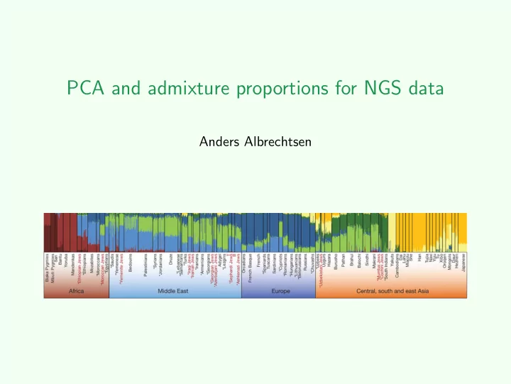
Anders Albrechtsen

Admixture model NGSadmix Introduction to PCA PCA for NGS

Ancient Eskimoa

aRasmussen et. al., Nature 2010

Figure: First principal components of selected populations.

Admixture model NGSadmix Introduction to PCA PCA for NGS

Admixture: Inuit vs. European

Admixture model NGSadmix Introduction to PCA PCA for NGS

26.5% European admixture in Greenland

Admixture model NGSadmix Introduction to PCA PCA for NGS

Admixture: PCA analysis

Admixture model NGSadmix Introduction to PCA PCA for NGS

What hope you get out of this session

Learning objectives

• Be able to understand the underlying model for PCA and admixture

analysis

• Understand the problem with genotype uncertainty for NGS data
• Learn some tricks and tools to overcome the problem
• Be able to do PCA and to infer ancestry proportions from NGS data

Admixture model NGSadmix Introduction to PCA PCA for NGS

Outline

1

Admixture model Intro to the problem Maximum likelihood (ML) solution based on called genotypes

2

NGSadmix ML inference based on genotype likelihoods

3

Introduction to PCA population structure and PCA Problems with PCA analysis NGS data

4

PCA for NGS The expectation of the covariance

Admixture model NGSadmix Introduction to PCA PCA for NGS

Basic problem

• Underlying assumption: All analyzed individuals have DNA that
• riginates from one or more of K source populations.
• Consequence: they will have some proportion of DNA from each of the K

populations; these proportions are called admixture proportions

• Examples with K=2:
• A dataset consisting of samples from two different populations
• Two populations that have mixed
• Goal: to infer overall admixture proportions (+ identify clusters)

Admixture model NGSadmix Introduction to PCA PCA for NGS

Overview of well known solutions

• Several methods:
• Bayesian: e.g. Structure (Pritchard et al. 2000, BABS - Mikko J

Sillanp

• Maximum Likelihood: e.g. Admixture (Alexander et al. 2009)
• They all base their inference on called genotypes and infer

1

Admixture proportions, Q

2

Allele frequencies for all loci for all K populations, F

Admixture model NGSadmix Introduction to PCA PCA for NGS

ML solution

• To find an ML solution we have to
• Define a model/likelihood function p(data|Q, F)
• Find an efficient way to find argmax

(Q,F)

p(data|Q, F)

• The latter is usually solved using EM which I will no focus on
• I will spend time describing the model/likelihood function

Admixture model NGSadmix Introduction to PCA PCA for NGS

Likelihood function (1 individual i, 1 diallelic locus j)

Assume K source populations and let

• Qi = (qi

1, qi 2, ..., qi K) be i’s genomewide admixture proportions

• Gij be the genotype of i in j (measured in counts of allele A)
• F j = (f j

1 , f j 2 , ..., f j K) denote the allele frequencies of allele A

Then

• for one of i’s alleles: p(allele|Qi, F j) = qi

1f j 1 + qi 2f j 2 + ...qi Kf j K = hij

• therefore assuming HWE we get the likelihood function:

p(Gij|Qi, F j) =    (hij)2 if Gij = 2, 2hij(1 − hij) if Gij = 1, (1 − hij)2 if Gij = 0.

Admixture model NGSadmix Introduction to PCA PCA for NGS

Likelihood function (N individuals, M diallelic loci)

• If we assume:
• the individuals are unrelated and thus independent
• loci are independent

we can write the likelihood as p(G|Q, F) =

N

• i

M

• j

p(Gij|Qi, F j) with G = (Gij), Q = (Q1, Q2, ...QN) and F = (F 1, F 2, ...F M).

• Based on this we can find ML estimates: ( ˆ

Q, ˆ F) = argmax

(Q,F)

p(G|Q, F). Very large number of parameters M× K + N × (K-1)

Admixture model NGSadmix Introduction to PCA PCA for NGS

reformulation of the likelhood

the likelihood - Gij = g 1

ij + g 2 ij

p(G|Q, F) =

N

• i

M

• j

p(Gij|Qi, F j) ∝

N

• i

M

• j

2

• d

p(g d

ij |Qi, F j)

=

N

• i

M

• j

2

• d
• A

p(g d

ij |Qi, F j, A)p(A|Qi, F j)

=

N

• i

M

• j

2

• d
• A

p(g d

ij |F j, A)p(A|Qi)

p(A|Qi) = qi

A and p(g d ij |F j, A) = f j AI0(g d ij ) + (1 − f j A)I1(g d ij )

Admixture model NGSadmix Introduction to PCA PCA for NGS

Some problems (NGS data, variable depth)

Admixture model NGSadmix Introduction to PCA PCA for NGS

Some problems (NGS data, variable depth)

Admixture model NGSadmix Introduction to PCA PCA for NGS

Genotype likelihoods

The genotype likelihood p(data | geno) Summarise the data in 10 genotype likelihoods

bases: TTTCCTTTTTTTTTTTTT quality score: BBGHSSBBTTTTGHRSBB

֌ A C G T A * * * * C * * * G * * T *

Admixture model NGSadmix Introduction to PCA PCA for NGS

Genotype likelihoods

The genotype likelihood p(data | geno) Summarise data for diallelic site

bases: TTTCCTTTTTTTTTTTTT quality score: BBGHSSBBTTTTGHRSBB

֌ p(data | geno = 0) 1 p(data | geno = 1) 2 p(data | geno = 2)

Admixture model NGSadmix Introduction to PCA PCA for NGS

Solution: NGSadmix

• Works on genotype likelihoods instead of called genotypes
• I.e. input is p(Xij|Gij) for all 3 possible values of Gij,

where Xij is NGS data for individual i at locus j

• The previous likelihood is extended from

p(G|Q, F) =

N

• i

M

• j

p(Gij|Qi, F j)

to

p(X|Q, F) =

N

• i

M

• j

p(Xij|Qi, F j) =

N

• i

M

• j
• Gij ∈{0,1,2}

p(Xij|Gij)p(Gij|Qi, F j)

• Note that for known genotypes the two are equivalent
• A solution is found using an EM-algorithm

Admixture model NGSadmix Introduction to PCA PCA for NGS

Solution: NGSadmix

• Does well even for low depth and variable depth data:

Admixture model NGSadmix Introduction to PCA PCA for NGS

Principal component analysis

SVD X = UDV T PCA for a covariance matrix MMT = C = VDV T

• The first principal component/eigenvector accounts for as much of

the variability in the data as possible

• Can be use to reduce the dimension of the data

Goal Capture the population structure in a low dimensional space

Admixture model NGSadmix Introduction to PCA PCA for NGS

Genotype data

Admixture model NGSadmix Introduction to PCA PCA for NGS

The first principal component

Admixture model NGSadmix Introduction to PCA PCA for NGS

Measure for pairwise differences

Identical by descent (IBS) matrix - used in MDS The average genotype distance between individuals pros fast cons Ignores allele frequency cons Problems with some kinds of missingness Covariance / correlation matrix - used in PCA pros good weighting scheme for each site cons Slower and cannot easily deal with any kind of missing data

Admixture model NGSadmix Introduction to PCA PCA for NGS

Approximation of the genotype covariance

M number of sites G genotypes G j genotypes for individual j G j

k genotypes for site k in individual j

fk allele frequency for site k Known genotypes - covariance between individuals i and ja

aPatterson N, Price AL, Reich D, plos genet. 2006

cov(G i, G j) = 1 M

M

• k=1

(G i

k − 2fk)(G j k − 2fk)

2fk(1 − fk) = 1 M ˜ G ˜ G T ˜ G i

k =

G i

k − 2fk

• 2fk(1 − fk)

var(Gk) = 2fk(1 − fk)

Admixture model NGSadmix Introduction to PCA PCA for NGS

IBS matrix

genotypes Assuming the genotypes are coded as {0, 1, 2} Commonly used distance measure d(G i

k, G j k) =

       if G i

k = G j k ∧ G i k = 1

1 if G i

k = G j k ∧ G i k = 1

1 if |G i

k − G j k| = 1

2 if |G i

k − G j k| = 2

IBS distance between individual i and j d(G i, G j) = 1 M

M

• k=1

d(G i

k, G j k)

Admixture model NGSadmix Introduction to PCA PCA for NGS

The two first principal component

−0.20 −0.15 −0.10 −0.05 0.00 0.05 0.10 0.15 −0.2 −0.1 0.0 0.1 PC 1 PC 2

• Pop 1

Pop 2 Pop 3

Admixture model NGSadmix Introduction to PCA PCA for NGS

Early use of PCA in genetics

Shown 1 PC at 400 locations Science 1978 Menozzi P, Piazza A, Cavalli-Sforza L. Data 38 loci

Admixture model NGSadmix Introduction to PCA PCA for NGS

PCA mania

Genetic map from PCAa

aNovembre et. al, nat genet. 2008

Eigenstrata

aPrice et. al, nat genet. 2008

Admixture model NGSadmix Introduction to PCA PCA for NGS

Sample size/information bias

Uneven sample sizes will bias both the distance and the pattern a

aMcVean G

PLoS Genet. (2009)

Admixture model NGSadmix Introduction to PCA PCA for NGS

Dealing with Missingness

Covariance matrix - Eigensoft a

aPatterson N, Price AL, Reich D, plos genet. 2006

If a genotype is missing then ˜ Gk i is set to zero

• E[˜

G i

k] = 0 for a random individual

• E[cov(G i, G j)] = 0 without relatedness or admixture.
• r a site is discarded
• Not possible for large samples
• Will likely cause ascertainment bias

IBS matrix The site is skipped for the pair of individuals

• Missingness must be random

Admixture model NGSadmix Introduction to PCA PCA for NGS

non random missingness

Major source Using multiple source of data

• Two SNP chips with not all individuals typed using both.
• Using SNP chip for some and sequencing for others

Minor sources

• Differential missingness between individuals
• Sequencing at different depths

Admixture model NGSadmix Introduction to PCA PCA for NGS

It is still kind of useful - and pretty

Ancient Eskimoa

aRasmussen et. al., Nature 2010

Figure: First principal components of selected populations.

Admixture model NGSadmix Introduction to PCA PCA for NGS

Genotype likelihoods

The genotype likelihood P(sequencing data | unobserved genotype) = P(X|G) Summarise data for diallelic site

bases: TTTCCTTTTTTTTTTTTT quality score: BBGHSSBBTTTTGHRSBB

֌ P(X | G = 0) 1 P(X | G = 1) 2 P(X | G = 2)

Admixture model NGSadmix Introduction to PCA PCA for NGS

PCA for NGS

the model based on GL

cov(G i, G j) = 1 M

M

• k=1
• {G1,G2}(G 1 − 2fk)(G 2 − 2fk)p(G 1, G 2|X j

k, X i k)

2fk(1 − fk) ,

Admixture model NGSadmix Introduction to PCA PCA for NGS

PCA for NGS

the model based on GLa

aSkotte, genet epi. 2012

cov(G i, G j) = 1 M

M

• k=1
• {G1,G2}(G 1 − 2fk)(G 2 − 2fk)p(G 1|X i

k)p(G 2|X j k)

2fk(1 − fk) ,

were p(G|X) is the posterior probability estimated using the allele frequency as a prior. assumption: p(G 1, G 2|X j

k, X i k) = p(G 1|X i k, fk)p(G 2|X j k, fk),

with p(G 1|X i

k, fk) ∝ p(X i k|G 1 k )p(G 1 k |fk)

motivation is the same as eigensoft

• E[˜

G i

k] = 0 for a random individual

• E[cov(G i, G j)] = 0 without relatedness or admixture.

Admixture model NGSadmix Introduction to PCA PCA for NGS

PCA for NGS

the model based on GLa

aSkotte, genet epi. 2012

cov(G i, G j) = 1 M

M

• k=1
• {G1,G2}(G 1 − 2fk)(G 2 − 2fk)p(G 1|X i

k)p(G 2|X j k)

2fk(1 − fk) ,

avg Depth per individual

Depth

1 2 3 4 −0.20 −0.15 −0.10 −0.05 0.00 0.05 0.10 0.15 −0.2 −0.1 0.0 0.1

Known genotypes

PC 1 PC 2

• Pop 1

Pop 2 Pop 3

−0.20 −0.15 −0.10 −0.05 0.00 0.05 0.10 −0.20 −0.10 0.00 0.05 0.10 0.15

E(G|f), Depth = 4

PC 1 PC 2

• Pop 1

Pop 2 Pop 3

Admixture model NGSadmix Introduction to PCA PCA for NGS

PCA for NGS, ascertainment corrected

Model that work without inferring variable sitesa

aFumagalli, et al, Genetics, 2013

cov(G i, G j) = 1 M

M

• k=1
• {G1,G2}(G 1 − 2fk)(G 2 − 2fk)p(G 1|X i

k)p(G 2|X j k)pk var

2fk(1 − fk) M

k′=1 pk′ var

,

were p(G|X) is the posterior probability estimated using the allele frequency as a prior

Admixture model NGSadmix Introduction to PCA PCA for NGS

The assumption of independents can be problematic

the model based on GLa

aSkotte, genet epi. 2012

cov(G i, G j) = 1 M

M

• k=1
• {G1,G2}(G 1 − 2fk)(G 2 − 2fk)p(G 1|X i

k)p(G 2|X j k)

2fk(1 − fk) ,

avg Depth per individual

Depth

5 10 15 20 −0.15 −0.10 −0.05 0.00 0.05 0.10 0.15 −0.20 −0.15 −0.10 −0.05 0.00 0.05 0.10

Known genotypes

PC 1 PC 2

• Pop 1

Pop 2 Pop 3

−0.15 −0.10 −0.05 0.00 0.05 0.10 0.15 −0.20 −0.10 0.00 0.05 0.10

E(G|f)

PC 1 PC 2

• Pop 1

Pop 2 Pop 3

Admixture model NGSadmix Introduction to PCA PCA for NGS

The problem under extreme depth differences

The assumption is valid under HWEa for unrelated individuals

aFumagalli, et al, Genetics, 2013

p(G 1, G 2|X j

k, X i k, fk) = p(G 1|X i k, fk)p(G 2|X j k, fk) assuming known allele

frequency

• The HWE assumption assumes no population structure!

One solution - use the IBS matrix or sample a single read d(g i

k, g j k) =

if g i

k = g j k

1 if g i

k = g j k

Admixture model NGSadmix Introduction to PCA PCA for NGS

IBS matrix not affected by depth bias

Admixture proportions

0.0 0.2 0.4 0.6 0.8 1.0 −0.15 −0.10 −0.05 0.00 0.05 −0.10 −0.05 0.00 0.05 0.10

known genotypes

PC 1 PC 2

• Pop 1

Pop 2 Pop 3

−0.15 −0.10 −0.05 0.00 0.05 −0.10 −0.05 0.00 0.05 0.10

Called genotypes

PC 1 PC 2

• Pop 1

Pop 2 Pop 3

avg Depth per individual

Depth 5 10 15 20 −0.15 −0.10 −0.05 0.00 0.05 −0.10 −0.05 0.00 0.05 0.10

E(G|f)

PC 1 PC 2

• Pop 1

Pop 2 Pop 3

−0.15 −0.10 −0.05 0.00 0.05 −0.10 −0.05 0.00 0.05 0.10

NGSadmix/admixRelate

PC 1 PC 2

• Pop 1

Pop 2 Pop 3

IBS matrix based

Admixture model NGSadmix Introduction to PCA PCA for NGS

The end

Conclusion

• Calling genotypes will cause major bias for PCA and Admixture
• Using genotype likelihoods instead can solve the problems

Time for exercises

Summary of EM results

To find the ML solution to log(L(θ)) =

• i

log  

j

p(Xi, Zj|θ)   , when

j θj = 1 and p(X|Z, θ) = p(X|Z) and p(Zj|θ) = θj

Q qi(Zj) = p(Zj|Xi, θ(n)) M θ(n+1)

j

=

• i qi(Zj)
• i
• j qi(Zj)

EM for ancestry

To find the ML solution to log(L(θ)) =

• i

log  

j

p(gi, Aj|θ)   , when

j qi j = 1 and p(g|A, Q) = p(g|A) and p(Aj|Q) = qj

Q (Q in bold is the EM q function) qi(Aj) =p(Aj|g 1

i , Q(n), f (n)) + p(Aj|g 2 i , Q(n), f (n))

p(Aj|g d

i , Q(n), f (n)) ∝p(g d i |A, F j)p(A|Qi) = qi A

• f j

AI0(g d ij ) + (1 − f j A)I1(g d ij )

• M

q(n+1)

j

=

• i qi(Aj)
• i
• j qi(Aj)

EM-algorithm (as written in paper)

f jk

n+1 =

N

i aijk

N

i aijk + N i bijk

, qik

n+1 =

1 2M

M

• j

(aijk + bijk) , where aijk = Gij qik

n f jk n

• k′ qik′

n f jk′ n

bijk = (2 − Gij) qik

n (1 − f jk n )

• k′ qik′

n (1 − f jk′ n )

.

EM-algorithm

f jk

n+1 =

N

i aijk

N

i aijk + N i bijk

, qik

n+1 =

1 2M

M

• j

(aijk + bijk) , where aijk = H(X ij|qik

n , f j. n )

qik

n f jk n

• k′ qik′

n f jk′ n

bijk = (2 − H(X ij|qik

n , f j. n ))

qik

n (1 − f jk n )

• k′ qik′

n (1 − f jk′ n )

. Without uncertainty H(X ij|qik

n , f j. n )) = G ij and with uncertainty

H(X ij|qik

n , f j. n )) =

• g∈{0,1,2} p(X ij|g)p(g|hij)g
• g∈{0,1,2} p(X ij|g)p(g|hij)

Accelerated EM algorithm

SQUAREM Two EM steps θ0

EM

→ θ1

EM

→ θ2 Calculate differences and steplength r = θ1 − θ0 v = θ2 − θ1 α = − r v Accelerated EM update θnew = θ0 − 2αr + α2v

Convergence of M algorithms

• 100

200 300 400 500 0.001 0.100 10.000 1000.000 Iterations log likelihood units from true maximum

• EM

Sq3 EM

ANGSD - Analysis of Next Generation Sequencing Data

ANGSD - Analysis of Next Generation Sequencing Data

Why angsd ANGSD can perform many analysis without the need to call genotypes and therefore will work for a large range of depth Often used for

• ABBABABA test/Dstatistics
• SFS reconstruction
• PCA/ADMIXTURE
• selection scans
• Error rate estimation
• contamination estimation

When not to use ANGSD you have high enough depth to call genotypes (GATK is better)

Data set in exercises

Data from 1000 Genomes

• 2500 individuals sequenced at low/medium depth (3-8X)
• mulitple populations

Human genomes

• 3Gb
• BAM file size 5Gb per X

Reduced genome

• 22 100k regions (one for each autosome)
• 1Mb region on chr5
• 3 x 10 individuals from
• African(YRI), European (CEU), East Asian (JPT)