PCA and Admixture proportions for low depth NGS data Anders - PowerPoint PPT Presentation

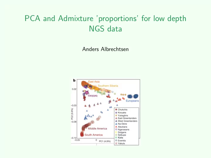
PCA and Admixture ’proportions’ for low depth NGS data Anders Albrechtsen

Structured populations analysis based on individual allele frequencies Analysis of low depth sequencing data Admixture proportions Individual allele frequencies (PCA) PCA thHan(40,919) alHan(80,714) SouthHan(20,969)

Structured populations analysis based on individual allele frequencies Admixture clustering /PCA - which is more informative?

Structured populations analysis based on individual allele frequencies This morning Structured populations 1 population structure and PCA analysis based on individual allele frequencies 2 Admixture proportions vs. PCA

Structured populations analysis based on individual allele frequencies PCA for NGS: Ancient Eskimo a a Rasmussen et. al. , 2010 Figure: First principal components of selected populations.

Structured populations analysis based on individual allele frequencies Genotype data 5 individuals, genotypes G: 5 individuals, allele counts SNP1 AG AG AG AA AA SNP1 1 1 1 0 0 SNP2 TT TA AA AT AA SNP2 0 1 2 1 2 SNP3 AA AC AC CC AC SNP3 2 1 1 0 1 SNP4 GG GG GC CC CC SNP4 0 0 1 2 2 SNP5 TT TC TC CC CC SNP5 2 1 1 0 0 SNP6 AA AA AC AC AC SNP6 0 0 1 1 1 SNP7 TT TT TC TC CC SNP7 2 2 1 1 0

Structured populations analysis based on individual allele frequencies singular value decomposition SVD - singular value decomposition G = UDV T • G (genotype matrix) does not have to be symmetric PCA for a covariance matrix (C) or pairwise distance √ DV T C = V • The first principal component/eigenvector accounts for as much of the variability in the data as possible • C is symmetric • Optimally the multidimensional data is identically distributed

Structured populations analysis based on individual allele frequencies IBS distances Total Distance Ind1 Ind2 Ind3 Ind4 Ind5 5 individuals Ind1 0 3 7 10 11 Ind2 3 0 4 7 8 SNP1 1 1 1 0 0 Ind3 7 4 0 5 4 SNP2 0 1 2 1 2 Ind4 10 7 5 0 3 SNP3 2 1 1 0 1 Ind5 11 8 4 3 0 SNP4 0 0 1 2 2 SNP5 2 1 1 0 0 SNP6 0 0 1 1 1 1 dimensional projection SNP7 2 2 1 1 0 Ind1 Ind2 Ind3 Ind4 Ind5 1st 0.65 0.36 -0.08 -0.4 -0.53

Structured populations analysis based on individual allele frequencies Approximation of the genotype covariance M number of sites G genotypes G j genotypes for individual j G j k genotypes for site k in individual j f k allele frequency for site k Known genotypes - covariance between individuals i and j a a Patterson N, Price AL, Reich D, plos genet. 2006 M k − 2 f k )( G j ( G i cov ( G i , G j ) = 1 k − 2 f k ) = 1 � G ˜ ˜ G T M 2 f k (1 − f k ) M k =1 G i k − 2 f k ˜ G i k = var ( G k ) = 2 f k (1 − f k ) , � 2 f k (1 − f k )

Structured populations analysis based on individual allele frequencies Dealing with Missingness Covariance matrix - Eigensoft a a Patterson N, Price AL, Reich D, plos genet. 2006 If a genotype is missing then ˜ G i k is set to zero • E [˜ G i k ] = 0 for a random individual • E [ cov ( G i , G j )] = 0 i.e. relatedness or population structure. or a site is discarded • Not possible for large samples • Will likely cause bias IBS matrix The site is skipped for the pair of individuals • Missingness must be random

Structured populations analysis based on individual allele frequencies Population frequencies causes depth bias Admixture proportions known genotypes Called genotypes 1.0 0.10 0.10 0.8 0.05 0.05 0.6 ● Pop 1 ● Pop 1 PC 2 PC 2 0.00 0.00 ● Pop 2 ● Pop 2 ● Pop 3 ● Pop 3 0.4 −0.05 −0.05 0.2 −0.10 −0.10 0.0 −0.15 −0.10 −0.05 0.00 0.05 −0.15 −0.10 −0.05 0.00 0.05 PC 1 PC 1 avg Depth per individual E(G|f) NGSadmix/admixRelate 20 0.10 0.10 15 0.05 0.05 ● Pop 1 ● Pop 1 Depth PC 2 0.00 PC 2 10 0.00 ● Pop 2 ● Pop 2 ● Pop 3 ● Pop 3 −0.05 −0.05 5 −0.10 −0.10 0 −0.15 −0.10 −0.05 0.00 0.05 −0.15 −0.10 −0.05 0.00 0.05 PC 1 PC 1

Structured populations analysis based on individual allele frequencies NGS framework for heterogenious samples Admixture aware priors Instead of a single allele frequency we will use a different prior for each individuals Admixture proportions priors individual allele frequency at site i: π i = q 1 i f 1 i + q 2 i f 2 i + ... + q k i f k i PCA based priors is also possible individual allele frequency predicted from the PCA

Structured populations analysis based on individual allele frequencies individual allele frequencies from PCA Figure: PCAngsd framework

Structured populations analysis based on individual allele frequencies 1000 Genomes - true genotypes Figure: 1000 Genomes data

Structured populations analysis based on individual allele frequencies 1000 Genomes - called genotypes from low depth Figure: 1000 Genomes data

Structured populations analysis based on individual allele frequencies 1000 Genomes - Genotype likelihood with frequency prior Figure: 1000 Genomes data

Structured populations analysis based on individual allele frequencies 1000 Genomes - Genotype likelihood with individuals frequency prior Figure: 1000 Genomes data

Structured populations analysis based on individual allele frequencies Admixture VS PCA indirect goal of both ADMIXTURE and PCA To predict the individual allele frequencies Π from lower dimensional matrices. E ( G ) = 2Π ADMIXTURE PCA K=N-1 G = 2 QF T K=N-1 ˜ G = UDV T K low Π ≈ QF T K low ˜ Π ≈ U [1: K ] DV T [1: K ] ADMIXTURE → PCA PCA → ADMIXTURE cov (˜ G i , ˜ argmin Q , F || Π − QF T || 2 G j ) = F (Π i m − f m )(Π j Solved with NMF with penalty m − f m ) 1 � M = m =1 M f m (1 − f m ) M ˜ G ˜ 1 G T

Structured populations analysis based on individual allele frequencies 140K chinese ultra low depth genomes PCA colored by province Figure: flash PCAngsd

Structured populations analysis based on individual allele frequencies Selection scan from PCA for NGS data FastPCA test statistic from Galinsky et al (2016) M Π m V k ) 2 ∼ χ 2 (2˜ D 2 k selection scan in > 140k Han chinese with low depth sequencing < 0 . 1 X thHan(40,919) alHan(80,714) SouthHan(20,969)

Structured populations analysis based on individual allele frequencies The end Conclusion • Calling genotypes can cause major bias for PCA and Admixture analysis • Using genotype likelihoods instead can solve the problems • Admixture analysis and PCA are related and can both be used to estimate individual allele frequencies • individual allele frequencies can be used for selection scans