h ( t ) y ( t ) x [ n ] h [ n ] y [ n ] Review of sampling property - PowerPoint PPT Presentation

Convolution Sum Overview Impulse Response • Review of time invariance x ( t ) h ( t ) y ( t ) x [ n ] h [ n ] y [ n ] • Review of sampling property • Discrete-time convolution sum • Recall that if x ( t ) = δ ( t ) or x [ n ] = δ [ n ] , the output of the system is called the impulse response • Two methods of visualizing • The impulse response is always denoted h ( t ) and h [ n ] • Some examples • For any input x ( t ) , it is possible to use h ( t ) to solve for y ( t ) • For any input x [ n ] , it is possible to use h [ n ] to solve for y [ n ] • This method is called convolution • This is a important concept • Is used to implement digital filters • The derivation of the continuous-time convolution integral is tricky • We will discuss the discrete-time convolution sum first J. McNames Portland State University ECE 222 Convolution Sum Ver. 1.06 1 J. McNames Portland State University ECE 222 Convolution Sum Ver. 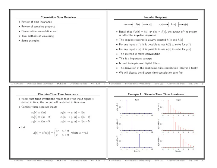1.06 2 Discrete-Time Time Invariance Example 1: Discrete-Time Time Invariance • Recall that time invariance means that if the input signal is Input Output 1 1 shifted in time, the output will be shifted in time also x 1 [n] = δ [n] y 1 [n] = h[n] • Consider three separate inputs 0.5 0.5 x 1 [ n ] ≡ δ [ n ] x 1 [ n ] → y 1 [ n ] = h [ n ] 0 0 −2 0 2 4 6 8 10 −2 0 2 4 6 8 10 x 2 [ n ] ≡ δ [ n − 2] x 2 [ n ] → y 2 [ n ] = h [ n − 2] 1 1 x 2 [n] = δ [n−2] y 2 [n] = h[n−2] x 3 [ n ] ≡ δ [ n − 5] x 3 [ n ] → y 3 [ n ] = h [ n − 5] 0.5 0.5 • Let � a n n ≥ 0 0 0 h [ n ] = a n u [ n ] = n < 0 , where a = 0 . 6 −2 0 2 4 6 8 10 −2 0 2 4 6 8 10 0 1 1 x 3 [n] = δ [n−5] y 3 [n] = h[n−5] 0.5 0.5 0 0 −2 0 2 4 6 8 10 −2 0 2 4 6 8 10 Time (n) Time (n) J. McNames Portland State University ECE 222 Convolution Sum Ver. 1.06 3 J. McNames Portland State University ECE 222 Convolution Sum Ver. 1.06 4

Example 1: MATLAB Code Example 1: MATLAB Code Continued a = 0.6; subplot(3,2,5); n = -2:10; x3 = (n==5); % Unit impulse centered at 5 subplot(3,2,1); h = stem(n,x3,’b’); x1 = (n==0); % Unit impulse centered at n=0 set(h(1),’Marker’,’.’); h = stem(n,x1,’b’); xlabel(’Time (n)’); set(h(1),’Marker’,’.’); ylabel(’x_3[n] = \delta[n-5]’); title(’Input’); box off; ylabel(’x_1[n] = \delta[n]’); xlim([min(n) max(n)]); box off; subplot(3,2,6); xlim([min(n) max(n)]); y3 = (a.^(n-5)).*(n>=5); % Unit impulse response h[n] subplot(3,2,2); h = stem(n,y3,’r’); y1 = (a.^n).*(n>=0); % Unit impulse response h[n] set(h(1),’Marker’,’.’); h = stem(n,y1,’r’); xlabel(’Time (n)’); set(h(1),’Marker’,’.’); ylabel(’y_3[n] = h[n-5]’); title(’Output’); box off; ylabel(’y_1[n] = h[n]’); xlim([min(n) max(n)]); box off; xlim([min(n) max(n)]); subplot(3,2,3); x2 = (n==2); % Unit impulse centered at n=2 h = stem(n,x2,’b’); set(h(1),’Marker’,’.’); ylabel(’x_2[n] = \delta[n-2]’); box off; xlim([min(n) max(n)]); subplot(3,2,4); y2 = (a.^(n-2)).*(n>=2); % Unit impulse response h[n] h = stem(n,y2,’r’); set(h(1),’Marker’,’.’); ylabel(’y_2[n] = h[n-2]’); box off; xlim([min(n) max(n)]); J. McNames Portland State University ECE 222 Convolution Sum Ver. 1.06 5 J. McNames Portland State University ECE 222 Convolution Sum Ver. 1.06 6 Discrete-Time Unit-Impulse Sampling Property Example 2: Unit-Impulse Sampling Property Recall from our earlier discussion of signal fundamentals that any • Any bounded discrete-time signal can be written as a sum of signal x [ n ] can be written as discrete-time impulses • For example, consider the following signal ∞ � x [ n ] = x [ k ] δ [ n − k ] ⎧ 1 n = 0 k = −∞ ⎪ ⎪ ⎪ − 1 n = 2 ∞ ⎨ � x [ n ] = = a k x k [ n ] 2 n = 5 ⎪ k = −∞ ⎪ ⎪ 0 otherwise ⎩ Side note: since δ [ n ] is an even signal, δ [ n ] = δ [ − n ] , we can also write • In terms of unit-impulses, this signal can also be expressed as this as ∞ x [ n ] = 1 · δ [ n ] − 1 · δ [ n − 2] + 2 · δ [ n − 5] � x [ n ] = x [ k ] δ [ k − n ] k = −∞ Though, this is not the conventional form. J. McNames Portland State University ECE 222 Convolution Sum Ver. 1.06 7 J. McNames Portland State University ECE 222 Convolution Sum Ver. 1.06 8

Example 3: Discrete-Time Unit Sampling Example Example 3: MATLAB Code n = -2:10; Example of Unit Sampling x1 = 1*(n==0); % Unit impulse centered at n=0 2 x2 = -1*(n==2); % Unit impulse centered at n=2 1 x3 = 2*(n==5); % Unit impulse centered at 0 x 1 [n] x = x1 + x2 + x3; % The original signal 0 X = [x1;x2;x3;x]; −1 for cnt = 1:4, −2 0 2 4 6 8 10 subplot(4,1,cnt); 2 plot([min(n) max(n)],[0 0],’k:’); hold on; 1 x 2 [n] h = stem(n,X(cnt,:),’b’); set(h(1),’Marker’,’.’); 0 hold off; −1 box off; −2 0 2 4 6 8 10 axis([min(n) max(n) min(x) max(x)]); 2 if cnt==1, ylabel(’x_1[n]’); 1 x 3 [n] title(’Example of Unit Sampling’); elseif cnt==2, 0 ylabel(’x_2[n]’); elseif cnt==3, −1 ylabel(’x_3[n]’); −2 0 2 4 6 8 10 elseif cnt==4, 2 ylabel(’x[n]’); 1 xlabel(’Time (n)’); x[n] end; 0 end; −1 −2 0 2 4 6 8 10 Time (n) J. McNames Portland State University ECE 222 Convolution Sum Ver. 1.06 9 J. McNames Portland State University ECE 222 Convolution Sum Ver. 1.06 10 Discrete-Time Convolution Sum Derived Discrete-Time Convolution Sum • Any discrete-time input signal x [ n ] can be expressed as a sum of x [ n ] = x 1 [ n ] + x 2 [ n ] + x 3 [ n ] = 1 · δ [ n ] − 1 · δ [ n − 2] + 2 · δ [ n − 5] scaled unit impulses by linearity, we know the output will be equal to the sum of the ∞ � x [ n ] = x [ k ] δ [ n − k ] outputs due to the application of x 1 [ n ] , x 2 [ n ] , and x 3 [ n ] alone. k = −∞ x [ n ] → y [ n ] = y 1 [ n ] + y 2 [ n ] + y 3 [ n ] • By linearity and time invariance , the output of the system is the Since scaled sum of outputs due to each unit impulse ∞ x 1 [ n ] ≡ δ [ n ] x 1 [ n ] → y 1 [ n ] = h [ n ] � x [ n ] → y [ n ] = h [ n ] ∗ x [ n ] = x [ k ] h [ n − k ] x 2 [ n ] ≡ − δ [ n − 2] x 2 [ n ] → y 2 [ n ] = − h [ n − 2] k = −∞ x 3 [ n ] ≡ 2 · δ [ n − 5] x 3 [ n ] → y 3 [ n ] = 2 · h [ n − 5] • This is called the discrete-time convolution sum Therefore, • This applies to all LTI discrete-time systems! y [ n ] = h [ n ] − h [ n − 2] + 2 · h [ n − 5] • If we know h [ n ] , then we can calculate y [ n ] for any input x [ n ] • Thus, h [ n ] completely characterizes LTI discrete-time systems J. McNames Portland State University ECE 222 Convolution Sum Ver. 1.06 11 J. McNames Portland State University ECE 222 Convolution Sum Ver. 1.06 12

Example 4: Discrete-Time Convolution Sum Example 4: MATLAB Code a = 0.6; Input Output n = -2:10; 2 2 x1 = 1*(n==0); % Unit impulse centered at n=0 x2 = -1*(n==2); % Unit impulse centered at n=2 1 1 x 1 [n] y 1 [n] x3 = 2*(n==5); % Unit impulse centered at 0 x = x1 + x2 + x3; % The original signal 0 0 y1 = 1*a.^(n-0).*(n>=0); −1 −1 y2 = -1*a.^(n-2).*(n>=2); y3 = 2*a.^(n-5).*(n>=5); −2 0 2 4 6 8 10 −2 0 2 4 6 8 10 2 2 y = y1 + y2 + y3; % The original signal X = [x1;x2;x3;x]; 1 1 x 2 [n] y 2 [n] Y = [y1;y2;y3;y]; for cnt = 1:4, 0 0 subplot(4,2,2*cnt-1); plot([min(n) max(n)],[0 0],’k:’); −1 −1 hold on; −2 0 2 4 6 8 10 −2 0 2 4 6 8 10 h = stem(n,X(cnt,:),’b’); 2 2 set(h(1),’Marker’,’.’); hold off; 1 1 x 3 [n] y 3 [n] box off; 0 0 axis([min(n) max(n) -1 2]); if cnt==1, −1 −1 ylabel(’x_1[n]’); −2 0 2 4 6 8 10 −2 0 2 4 6 8 10 title(’Input’); 2 2 elseif cnt==2, ylabel(’x_2[n]’); 1 1 elseif cnt==3, x[n] y[n] ylabel(’x_3[n]’); 0 0 elseif cnt==4, ylabel(’x[n]’); −1 −1 xlabel(’Time (n)’); −2 0 2 4 6 8 10 −2 0 2 4 6 8 10 end; Time (n) Time (n) J. McNames Portland State University ECE 222 Convolution Sum Ver. 1.06 13 J. McNames Portland State University ECE 222 Convolution Sum Ver. 1.06 14 Example 4: MATLAB Code Continued Discrete-Time Convolution Derivation Summary subplot(4,2,2*cnt); plot([min(n) max(n)],[0 0],’k:’); x [ n ] h [ n ] y [ n ] hold on; h = stem(n,Y(cnt,:),’r’); set(h(1),’Marker’,’.’); Definition of h [ n ] hold off; box off; δ [ n ] h [ n ] h [ n ] axis([min(n) max(n) -1 2]); if cnt==1, ylabel(’y_1[n]’); Time Invariance title(’Output’); elseif cnt==2, δ [ n − k ] h [ n ] h [ n − k ] ylabel(’y_2[n]’); elseif cnt==3, ylabel(’y_3[n]’); Linearity elseif cnt==4, ylabel(’y[n]’); xlabel(’Time (n)’); x [ k ] δ [ n − k ] h [ n ] x [ k ] h [ n − k ] end; end; Linearity � + ∞ Σ + ∞ h [ n ] k = - ∞ x [ k ] h [ n − k ] k = - ∞ x [ k ] δ [ n − k ] Definition of δ [ n ] Σ + ∞ x [ n ] h [ n ] k = - ∞ x [ k ] h [ n − k ] J. McNames Portland State University ECE 222 Convolution Sum Ver. 1.06 15 J. McNames Portland State University ECE 222 Convolution Sum Ver. 1.06 16