Machine Learning II: Beyond Decision Trees AI Class 15 (Ch. - - PDF document

1

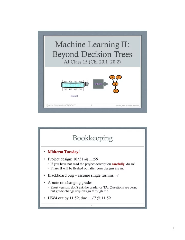
Machine Learning II: Beyond Decision Trees

AI Class 15 (Ch. 20.1–20.2)

Cynthia Matuszek – CMSC 671

Material from Dr. Marie desJardin,

1 Data D

Inducer C A E B

E[1] B[1] A[1] C[1] ⋅ ⋅ ⋅ ⋅ ⋅ ⋅ ⋅ ⋅ E[M] B[M] A[M] C[M] ⎡ ⎣ ⎢ ⎢ ⎢ ⎢ ⎤ ⎦ ⎥ ⎥ ⎥ ⎥

Bookkeeping

• Midterm Tuesday!
• Project design: 10/31 @ 11:59
• If you have not read the project description carefully, do so!
• Phase II will be fleshed out after your designs are in.
• Blackboard bug – assume single turnins. :-/
• A note on changing grades
• Short version: don’t ask the grader or TA. Questions are okay,

but grade change requests go through me

• HW4 out by 11:59; due 11/7 @ 11:59

2

2

Today’s Class

• Extensions to Decision Trees
• Sources of error
• Evaluating learned models
• Bayesian Learning
• MLA, MLE, MAP
• Bayesian Networks I

3

Information Gain

• Concept: make decisions that increase the

homogeneity of the data subsets (for outcomes)

• Good:

Bad:

• Information gain is based on:
• Decrease in entropy
• After a dataset is split on an attribute.
• à High homogeneity – e.g., likelihood samples will

have the same class (outcome)

4

3

Extensions of the Decision Tree Learning Algorithm

• Using gain ratios
• Real-valued data
• Noisy data and overfitting
• Generation of rules
• Setting parameters
• Cross-validation for experimental validation of performance
• C4.5 is an extension of ID3 that accounts for unavailable

values, continuous attribute value ranges, pruning of decision trees, rule derivation, and so on

7

Using Gain Ratios

• Information gain favors attributes with a large number
• f values
• If we have an attribute D that has a distinct value for each

record, then Info(D,T) is 0, thus Gain(D,T) is maximal

• To compensate, use the following ratio instead of Gain:

GainRatio(D,T) = Gain(D,T) / SplitInfo(D,T)

• SplitInfo(D,T) is the information due to the split of T on

the basis of value of categorical attribute D

SplitInfo(D,T) = I(|T1|/|T|, |T2|/|T|, .., |Tm|/|T|)

where {T1, T2, .. Tm} is the partition of T induced by value

• f D

8

4

Real-Valued Data

• Select a set of thresholds defining intervals
• Each interval becomes a discrete value of the attribute
• How?
• Use simple heuristics…
• Always divide into quartiles
• Use domain knowledge…
• Divide age into infant (0-2), toddler (3 - 5), school-aged (5-8)
• Or treat this as another learning problem
• Try a range of ways to discretize the continuous variable and see

which yield “better results” w.r.t. some metric

• E.g., try midpoint between every pair of values

11

Noisy Data

• Many kinds of “noise” can occur in the examples:
• Two examples have same attribute/value pairs, but

different classifications

• Some values of attributes are incorrect
• Errors in the data acquisition process, the preprocessing phase, //
• Classification is wrong (e.g., + instead of -) because of

some error

• Some attributes are irrelevant to the decision-making

process, e.g., color of a die is irrelevant to its outcome

• Some attributes are missing (are pangolins bipedal?)

12

5

Overfitting

• Overfitting: coming up with a model that is TOO specific to

your training data

• Does well on training set but not new data
• How can this happen?
• Too little training data
• Irrelevant attributes
• high-dimensional (many attributes) hypothesis space à meaningless

regularity in the data irrelevant to important, distinguishing features

• Fix by pruning lower nodes in the decision tree
• For example, if Gain of the best attribute at a node is below a threshold,

stop and make this node a leaf rather than generating children nodes

13

Pruning Decision Trees

• Replace a whole subtree by a leaf node
• If: a decision rule establishes that he expected error rate in the subtree is

greater than in the single leaf. E.g.,

• Training: one training red success and two training blue failures
• Test: three red failures and one blue success
• Consider replacing this subtree by a single Failure node. (leaf)
• After replacement we will have only two errors instead of five:

Color

1 success 0 failure 0 success 2 failures red blue

Color

1 success 3 failure 1 success 1 failure red blue 2 success 4 failure

FAILURE

Training Test Pruned

14

6

Converting Decision Trees to Rules

• It is easy to derive a rule set from a decision tree:
• Write a rule for each path in the decision tree from the root to a leaf
• Left-hand side is label of nodes and labels of arcs
• The resulting rules set can be simplified:
• Let LHS be the left hand side of a rule
• Let LHS’ be obtained from LHS by eliminating some conditions
• We can replace LHS by LHS’ in this rule if the subsets of the training

set that satisfy respectively LHS and LHS’ are equal

• A rule may be eliminated by using metaconditions such as

“if no other rule applies”

15

Measuring Model Quality

• How good is a model?
• Predictive accuracy
• False positives / false negatives for a given cutoff threshold
• Loss function (accounts for cost of different types of errors)
• Area under the (ROC) curve
• Minimizing loss can lead to problems with overfitting

17

7

Measuring Model Quality

• Training error
• Train on all data; measure error on all data
• Subject to overfitting (of course we’ll make good

predictions on the data on which we trained!)

• Regularization
• Attempt to avoid overfitting
• Explicitly minimize the complexity of the function while

minimizing loss

• Tradeoff is modeled with a regularization parameter

18

Cross-Validation

• Holdout cross-validation:
• Divide data into training set and test set
• Train on training set; measure error on test set
• Better than training error, since we are measuring

generalization to new data

• To get a good estimate, we need a reasonably large test set
• But this gives less data to train on, reducing our model

quality!

19

8

Cross-Validation, cont.

• k-fold cross-validation:
• Divide data into k folds
• Train on k-1 folds, use the kth fold to measure error
• Repeat k times; use average error to measure generalization

accuracy

• Statistically valid and gives good accuracy estimates
• Leave-one-out cross-validation (LOOCV)
• k-fold cross validation where k=N (test data = 1 instance!)
• Quite accurate, but also quite expensive, since it requires

building N models

20

Chapter 20.1-20.2

Bayesian Learning

Some material adapted from lecture notes by Lise Getoor and Ron Parr

26

9

Naïve Bayes

• Use Bayesian modeling
• Make the simplest possible independence

assumption:

• Each attribute is independent of the values of the other

attributes, given the class variable

• In our restaurant domain: Cuisine is independent of

Patrons, given a decision to stay (or not)

27

Bayesian Formulation

• The probability of class C given F1, ..., Fn

p(C | F1, ..., Fn) = p(C) p(F1, ..., Fn | C) / P(F1, ..., Fn) = α p(C) p(F1, ..., Fn | C)

• Assume that each feature Fi is conditionally independent of the
• ther features given the class C. Then:

p(C | F1, ..., Fn) = α p(C) Πi p(Fi | C)

• We can estimate each of these conditional probabilities from the
• bserved counts in the training data:

p(Fi | C) = N(Fi ∧ C) / N(C)

• One subtlety of using the algorithm in practice: When your estimated

probabilities are zero, ugly things happen

• The fix: Add one to every count (aka “Laplacian smoothing”)

28

10

Naive Bayes: Example

• p(Wait | Cuisine, Patrons, Rainy?)

= α p(Cuisine ∧ Patrons ∧ Rainy? | Wait) = α p(Wait) p(Cuisine | Wait) p(Patrons | Wait) p(Rainy? | Wait) naive Bayes assumption: is it reasonable?

29

Naive Bayes: Analysis

• Naïve Bayes is amazingly easy to implement (once

you understand the bit of math behind it)

• Naïve Bayes can outperform many much more

complex algorithms—it’s a baseline that should pretty much always be used for comparison

• Naive Bayes can’t capture interdependencies

between variables (obviously)—for that, we need Bayes nets!

30

11

Learning Bayesian Networks

31

Bayesian Learning: Bayes’ Rule

• Given some model space (set of hypotheses hi) and

evidence (data D):

• P(hi|D) = α P(D|hi) P(hi)
• We assume observations are independent of each other,

given a model (hypothesis), so:

• P(hi|D) = α ∏j P(dj|hi) P(hi)
• To predict the value of some unknown quantity X

(e.g., the class label for a future observation):

• P(X|D) = ∑i P(X|D, hi) P(hi|D) = ∑i P(X|hi) P(hi|D)

These are equal by our independence assumption

32

12

Bayesian Learning, 3 Ways

• BMA (Bayesian Model Averaging)
• Don’t just choose one hypothesis; instead, make predictions based on

the weighted average of all hypotheses (or some set of best hypotheses)

• MAP (Maximum A Posteriori) hypothesis
• Choose hypothesis with highest a posteriori probability, given data
• Maximize p(hi | D)
• Generally easier than Bayesian learning
• Closer to Bayesian prediction as more data arrives
• MLE (Maximum Likelihood Estimate)
• Assume all hypotheses are equally likely a priori; best hypothesis

maximizes the likelihood (i.e., probability of data given hypothesis)

• Maximize p(D | hi)

33

Bayesian Learning

• BMA (Bayesian Model Averaging) –

average predictions of hypotheses

• MAP (Maximum A Posteriori) hypothesis –

Maximize p(hi | D)

• MLE (Maximum Likelihood Estimate) –

Maximize p(D | hi)

• MDL (Minimum Description Length) principle: Use

some encoding to model the complexity of the hypothesis, and the fit of the data to the hypothesis, then minimize the overall description of hi + D

34

13

Learning Bayesian Networks

• Given training set
• Find B that best matches D
• model selection
• parameter estimation

]} [ ],..., 1 [ { M x x D =

Data D

Inducer C A E B

E[1] B[1] A[1] C[1] ⋅ ⋅ ⋅ ⋅ ⋅ ⋅ ⋅ ⋅ E[M] B[M] A[M] C[M] ⎡ ⎣ ⎢ ⎢ ⎢ ⎢ ⎤ ⎦ ⎥ ⎥ ⎥ ⎥ 35

Parameter Estimation

• Assume known structure
• Goal: estimate BN parameters q
• entries in local probability models, P(X | Parents(X))
• A good parameterization q is likely to generate
• bserved data:
• Maximum Likelihood Estimation (MLE) Principle:

Choose q* so as to maximize L

∏

= =

m

m x P D P D L ) | ] [ ( ) | ( ) : ( θ θ θ

36

i.i.d. samples independent and identically distributed (i.i.d.) if each random variable has the same probability distribution as the

• thers and all are mutually independent

14

Parameter Estimation II

• The likelihood decomposes according to the structure of the

network

→ we get a separate estimation task for each parameter

• The MLE (maximum likelihood estimate) solution:
• for each value x of a node X
• and each instantiation u of Parents(X)
• Just need to collect the counts for every combination of parents and

children observed in the data

• MLE is equivalent to an assumption of a uniform prior over

parameter values

) ( ) , (

* |

u N u x N

u x =

θ

sufficient statistics

37

Sufficient Statistics: Example

) ( ) , (

* |

u N u x N

u x =

θ

• Why are the counts sufficient?

Earthquake Burglary Alarm Moon-phase Light-level θ*

A | E, B = N(A, E, B) / N(E, B) 38

15

Model Selection

Goal: Select the best network structure, given the data Input:

• Training data
• Scoring function

Output:

• A network that maximizes the score

39

Handling Missing Data

• Suppose that in some cases, we observe

earthquake, alarm, light-level, and moon-phase, but not burglary

• Should we throw that data away??
• Idea: Guess the missing values

based on the other data

Earthquake Burglary Alarm Moon-phase Light-level

44

16

EM (Expectation Maximization)

• Guess probabilities for nodes with missing values

(e.g., based on other observations)

• Compute the probability distribution over the

missing values, given our guess

• Update the probabilities based on the guessed

values

• Repeat until convergence

45

EM Example

• Suppose we have observed Earthquake and Alarm but

not Burglary for an observation on November 27

• We estimate the CPTs based on the rest of the data
• We then estimate P(Burglary) for November 27 from

those CPTs

• Now we recompute the

CPTs as if that estimated value had been observed

• Repeat until convergence!

Earthquake Burglary Alarm

46