Machine Learning III: Beyond Decision Trees Extensions to Decision - PDF document

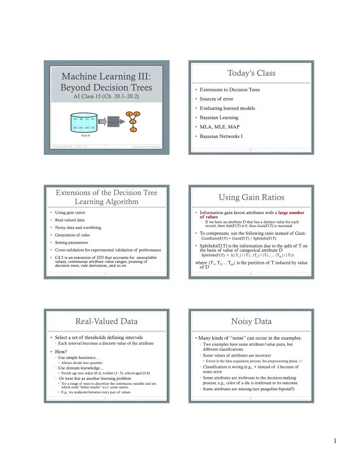
Today’s Class Machine Learning III: Beyond Decision Trees • Extensions to Decision Trees AI Class 15 (Ch. 20.1–20.2) • Sources of error • Evaluating learned models B E • Bayesian Learning ⎡ ⎤ E [1] B [1] A [1] C [1] ⎢ ⎥ Inducer A ⎢ ⋅ ⋅ ⋅ ⋅ ⎥ ⎢ ⋅ ⋅ ⋅ ⋅ ⎥ • MLA, MLE, MAP ⎢ ⎥ E [ M ] B [ M ] A [ M ] C [ M ] ⎣ ⎦ C • Bayesian Networks I Data D Cynthia Matuszek – CMSC 671 1 Material from Dr. Marie desJardin, 2 Extensions of the Decision Tree Using Gain Ratios Learning Algorithm • Using gain ratios • Information gain favors attributes with a large number of values • Real-valued data • If we have an attribute D that has a distinct value for each record, then Info (D,T) is 0, thus Gain (D,T) is maximal • Noisy data and overfitting • To compensate, use the following ratio instead of Gain: • Generation of rules GainRatio(D,T) = Gain(D,T) / SplitInfo(D,T) • Setting parameters • SplitInfo(D,T) is the information due to the split of T on • Cross-validation for experimental validation of performance the basis of value of categorical attribute D SplitInfo(D,T) = I(|T 1 |/|T|, |T 2 |/|T|, .., |T m |/|T|) • C4.5 is an extension of ID3 that accounts for unavailable values, continuous attribute value ranges, pruning of where {T 1 , T 2 , .. T m } is the partition of T induced by value decision trees, rule derivation, and so on of D 3 4 Real-Valued Data Noisy Data • Select a set of thresholds defining intervals • Many kinds of “noise” can occur in the examples: • Each interval becomes a discrete value of the attribute • Two examples have same attribute/value pairs, but different classifications • How? • Some values of attributes are incorrect • Use simple heuristics… • Errors in the data acquisition process, the preprocessing phase, // • Always divide into quartiles • Classification is wrong (e.g., + instead of -) because of • Use domain knowledge… some error • Divide age into infant (0-2), toddler (3 - 5), school-aged (5-8) • Some attributes are irrelevant to the decision-making • Or treat this as another learning problem process, e.g., color of a die is irrelevant to its outcome • Try a range of ways to discretize the continuous variable and see which yield “better results” w.r.t. some metric • Some attributes are missing (are pangolins bipedal?) • E.g., try midpoint between every pair of values 5 6 1

Overfitting Pruning Decision Trees • Replace a whole subtree by a leaf node • Overfitting: coming up with a model that is TOO specific to your training data • If: a decision rule establishes that he expected error rate in the subtree is greater than in the single leaf. E.g., • Does well on training set but not new data • Training: one training red success and two training blue failures • How can this happen? • Test: three red failures and one blue success • Too little training data • Consider replacing this subtree by a single Failure node. (leaf) • After replacement we will have only two errors instead of five: • Irrelevant attributes • high-dimensional (many attributes) hypothesis space à meaningless Pruned Test Training Color regularity in the data irrelevant to important, distinguishing features Color FAILURE • Fix by pruning lower nodes in the decision tree red red blue blue 2 success • For example, if Gain of the best attribute at a node is below a threshold, 1 success 4 failure 0 success 1 success 1 success stop and make this node a leaf rather than generating children nodes 1 failure 2 failures 3 failure 0 failure 7 8 Converting Decision Trees to Rules Measuring Model Quality • It is easy to derive a rule set from a decision tree: • How good is a model? • Write a rule for each path in the decision tree from the root to a leaf • Predictive accuracy • Left-hand side is label of nodes and labels of arcs • False positives / false negatives for a given cutoff threshold • Loss function (accounts for cost of different types of errors) • The resulting rules set can be simplified: • Area under the (ROC) curve • Let LHS be the left hand side of a rule • Minimizing loss can lead to problems with overfitting • Let LHS’ be obtained from LHS by eliminating some conditions • We can replace LHS by LHS’ in this rule if the subsets of the training set that satisfy respectively LHS and LHS’ are equal • A rule may be eliminated by using metaconditions such as “if no other rule applies” 9 11 Measuring Model Quality Cross-Validation • Training error • Holdout cross-validation: • Train on all data; measure error on all data • Divide data into training set and test set • Subject to overfitting (of course we’ll make good • Train on training set; measure error on test set predictions on the data on which we trained!) • Better than training error, since we are measuring generalization to new data • Regularization • To get a good estimate, we need a reasonably large test set • Attempt to avoid overfitting • But this gives less data to train on, reducing our model • Explicitly minimize the complexity of the function while quality! minimizing loss • Tradeoff is modeled with a regularization parameter 12 13 2

Cross-Validation, cont. Bayesian Learning • k-fold cross-validation: • Divide data into k folds • Train on k-1 folds, use the k th fold to measure error • Repeat k times; use average error to measure generalization accuracy Chapter 20.1-20.2 • Statistically valid and gives good accuracy estimates • Leave-one-out cross-validation (LOOCV) • k -fold cross validation where k=N (test data = 1 instance!) • Quite accurate, but also quite expensive, since it requires building N models Some material adapted from lecture notes by Lise Getoor and Ron Parr 15 14 Naïve Bayes Bayesian Formulation • The probability of class C given F 1 , ..., F n • Use Bayesian modeling p(C | F 1 , ..., F n ) = p(C) p(F 1 , ..., F n | C) / P(F 1 , ..., F n ) � = α p(C) p(F 1 , ..., F n | C) • Make the simplest possible independence assumption: • Assume that each feature F i is conditionally independent of the other features given the class C. Then: • Each attribute is independent of the values of the other p(C | F 1 , ..., F n ) = α p(C) Π i p(F i | C) attributes, given the class variable • We can estimate each of these conditional probabilities from the • In our restaurant domain: Cuisine is independent of observed counts in the training data: Patrons, given a decision to stay (or not) p(F i | C) = N(F i ∧ C) / N(C) • One subtlety of using the algorithm in practice: When your estimated probabilities are zero, ugly things happen • The fix: Add one to every count (aka “Laplacian smoothing”) 16 17 Naive Bayes: Example Naive Bayes: Analysis • Naïve Bayes is amazingly easy to implement (once • p(Wait | Cuisine, Patrons, Rainy?) � you understand the bit of math behind it) = α p(Cuisine ∧ Patrons ∧ Rainy? | Wait) � = α p(Wait) p(Cuisine | Wait) p(Patrons | Wait) � • Naïve Bayes can outperform many much more p(Rainy? | Wait) complex algorithms—it’s a baseline that should naive Bayes assumption: is it reasonable? pretty much always be used for comparison • Naive Bayes can’t capture interdependencies between variables (obviously)—for that, we need Bayes nets! 18 19 3