
SLIDE 1
Orthogonality Defined Two non-periodic power signals x1(t) and x2(t) are orthogonal if and
- nly if
lim
T →∞
1 2T T
−T
x1(t)x∗
2(t) dt = 0
- J. McNames
Portland State University ECE 223 CT Fourier Transform
- Ver. 1.24
3
Overview of Continuous-Time Fourier Transform Topics
- Definition
- Compare & contrast with Laplace transform
- Conditions for existence
- Relationship to LTI systems
- Examples
- Ideal lowpass filters
- Relationship to DTFS
- J. McNames
Portland State University ECE 223 CT Fourier Transform
- Ver. 1.24
1
Orthogonality of Complex Sinusoids Consider two (possibly non-harmonic) complex sinusoids x1(t) = ejω1t x2(t) = ejω2t Are they orthogonal? lim
T →∞
1 2T T
−T
x1(t)x∗
2(t) = lim N→∞
1 2T T
−T
ejω1te−jω2t dt = lim
N→∞
1 2T T
−T
ej(ω1−ω2)t dt =
- 1
ω1 = ω2 Otherwise
- J. McNames
Portland State University ECE 223 CT Fourier Transform
- Ver. 1.24
4
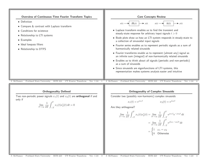
Core Concepts Review H(s)
x(t) y(t)
h(t)
x(t) y(t)
- Laplace transform enables us to find the transient and
steady-state response for arbitrary input signals t > 0
- Bode plots show us how an LTI system responds in steady-state to
a collection of sinusoidal input signals
- Fourier series enables us to represent periodic signals as a sum of
harmonically related sinusoids
- Fourier transforms enable us to represent (almost any) signal as
an infinite sum (integral) of non-harmonically related sinusoids
- Enables us to think about all signals (periodic and non-periodic)
as a sum of sinusoids
- Since sinusoids are eigenfunctions of LTI systems, this
representation makes systems analysis easier and intuitive
- J. McNames
Portland State University ECE 223 CT Fourier Transform
- Ver. 1.24