
SLIDE 1
1
SA-1
CSE-571 Robotics
Bayes Filters
GP-Based WiFi Sensor Model
Mean Variance
10/6/16 2 CSE-571: Probabilistic Robotics
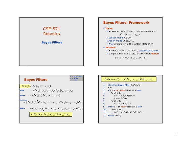
Bayes Filters: Framework
- Given:
- Stream of observations z and action data u:
- Sensor model P(z|x).
- Action model P(x|u,x).
- Prior probability of the system state P(x).
- Wanted:
- Estimate of the state X of a dynamical system.
- The posterior of the state is also called Belief:
) , , , | ( ) (
1 2 1 t t t t
z u z u x P x Bel
- =
! } , , , {
1 2 1 t t t
z u z u d
- =
!
Bayes Filters
) , , , | ( ) , , , , | (
1 1 1 1 t t t t t
u z u x P u z u x z P ! ! h =
Bayes z = observation u = action x = state
) , , , | ( ) (
1 1 t t t t
z u z u x P x Bel ! =
Markov
) , , , | ( ) | (
1 1 t t t t
u z u x P x z P ! h =
1 1 1
) ( ) , | ( ) | (
- ò
=
t t t t t t t
dx x Bel x u x P x z P h
Markov
1 1 1 1 1
) , , , | ( ) , | ( ) | (
- ò
=
t t t t t t t t
dx u z u x P x u x P x z P ! h
= η P(zt | xt ) P(xt | u1,z1,…,ut,xt−1)
∫
P(xt−1 | u1,z1,…,ut ) dxt−1
Total prob.
Bayes Filter Algorithm
1.
Algorithm Bayes_filter( Bel(x),d ): 2. n=0 3. If d is a perceptual data item z then 4. For all x do 5. 6. 7. For all x do 8. 9. Else if d is an action data item u then 10. For all x do 11. 12. Return Bel’(x)
) ( ) | ( ) ( ' x Bel x z P x Bel = ) ( ' x Bel + =h h ) ( ' ) ( '
1
x Bel x Bel
- =h
Bel'(x) = P(x | u,x')
∫
Bel(x') dx'
1 1 1
) ( ) , | ( ) | ( ) (
- ò
=
t t t t t t t t