Bel ( x t ) = P ( z t | x t ) P ( x t | u t 1 , x t 1 ) Bel ( x t - - PDF document

1

Lecture 15: Action and Sensor Models

CS 344R/393R: Robotics Benjamin Kuipers

Action and Sensor Models

• The Markov localization equation depends
• n two types of knowledge about the robot.
• The action model: P(xt | ut-1, xt-1)

– Given a state xt and odometry ut, the distribution over possible next states xt+1

• The sensor model: P(zt | xt)

– Given a state xt, the distribution over possible sensor images zt.

Bel(xt) = P(zt | xt) P(xt | ut1,xt1)

• Bel(xt1) dxt1

Interpolate Observation Times

• Odometry ut and laser

scans zt actually arrive at slightly different times.

• Interpolate to give

estimated odometry ut′ at the same time as the laser scan zt.

z1 z2 z3 u1 u2 u3 z1 z2 z3 u1’ u2’ u3’

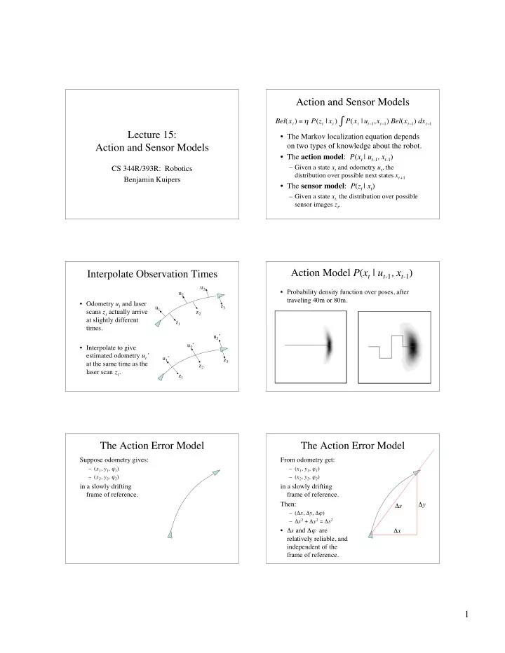
Action Model P(xt | ut-1, xt-1)

• Probability density function over poses, after

traveling 40m or 80m.

The Action Error Model

Suppose odometry gives:

– (x1, y1, ϕ1) – (x2, y2, ϕ2)

in a slowly drifting frame of reference.

The Action Error Model

From odometry get:

– (x1, y1, ϕ1) – (x2, y2, ϕ2)

in a slowly drifting frame of reference. Then:

– (Δx, Δy, Δϕ) – Δx2 + Δy2 = Δs2

• Δs and Δϕ are

relatively reliable, and independent of the frame of reference. Δx Δy Δs

2

The Action Error Model

From odometry get:

– (x1, y1, ϕ1) – (x2, y2, ϕ2)

in a slowly drifting frame

• f reference.

Then:

– (Δx, Δy, Δϕ) – Δx2 + Δy2 = Δs2

and:

– α = atan2(Δy,Δx)−ϕ1 – (Measure angle counter- clockwise from x-axis)

Δx Δy Δs Δϕ

α

The Action Error Model

From odometry get:

– (x1, y1, ϕ1) – (x2, y2, ϕ2) – (Δx, Δy, Δϕ) – Δx2 + Δy2 = Δs2 – α = atan2(Δy,Δx)−ϕ1

• Model the action as:

– Turn(α) – Travel(Δs) – Turn(Δϕ−α)

Δx Δy Δs Δϕ

α Δϕ−α

The Action Error Model

• Model the action as:

– Turn(α + ε1) – Travel(Δs + ε2) – Turn(Δϕ− α + ε3)

where

− ε1 ~ N(0, k1α) − ε2 ~ N(0, k2 Δs) − ε3 ~ N(0, k1 (Δϕ− α))

• This combines three

Gaussian errors.

– Std dev proportional to action magnitude

Δs

α Δϕ−α

Tune the Action Error Model

• Model the action as:

– Turn(α + ε1) – Travel(Δs + ε2) – Turn(Δϕ− α + ε3)

where

− ε1 ~ N(0, k1α) − ε2 ~ N(0, k2 Δs) − ε3 ~ N(0, k1 (Δϕ− α))

• Tune the model by

finding k1 and k2.

• Compute error

between:

– odometry observed – odometry corrected by localization.

• Divide by turn or

travel magnitude.

• Compute standard

deviations

– k1 = 1.0 – k2 = 0.4

The Action Model P(xt | ut-1, xt-1)

• Given a small motion ut-1 = (α, Δs, Δϕ−α)

where

− ε1 ~ N(0, k1α) − ε2 ~ N(0, k2 Δs) − ε3 ~ N(0, k1 (Δϕ− α))

xt yt t

• =

xt1 yt1 t1

• +

(s + 2)cos(t1 + + 1) (s + 2)sin(t1 + + 1) + 1 + 3

• Sensor Model P(zt | xt)
• For a given range measurement at a given

location xt in the map:

3

Laser Rangefinder Scan zt Density P(zt | xt) by Location Computing P(zt | xt)

• Image probabilities are too small to be

meaningful:

• But log probabilities can be accumulated

– without numerical underflow.

P(zt | xt) = P(ray(i) = di | xt)

i=1 180

• logP(zt | xt) =

logP(ray(i) = di | xt)

i=1 180

• Q: Didn’t we use log odds before?
• Yes, but that was in the occupancy grid.

– It is useful as a way to represent P(occ(i,j)) – Certainty on either side of ignorance

• Here, we’re doing Markov localization.
• We need to compare values of P(zt | xt).

– Odds would just be a distraction – Log helps us avoid numerical underflow

Bel(xt) = P(zt | xt) P(xt | ut1,xt1)

• Bel(xt1) dxt1

P(ray(i) = di | xt) Computing log P(ray(i) = di | xt)

• If ray(i) terminates at the first obstacle:

log P(ray(i)=di | xt) = −4

• If ray(i) terminates before an obstacle:

log P(ray(i)=di | xt) = −8

• If ray(i) terminates after an obstacle:

log P(ray(i)=di | xt) = −12

• Add them up for i=1 to 180.

– log P(zt | xt) totals between −720 and −2160 – Exponentiating would give zero!

logP(zt | xt) = logP(ray(i) = di | xt)

i=1 180

4

How Can We Normalize?

• To compute η, we must add un-normalized

values, each with log much less than -720.

– Exponentiating would give zero for every one!

• Solution:

– Adjust by adding the largest log P to all values. – Exponentiate. The largest values remain non-zero. – Then normalize, which divides out the adjustment. – Underflow only eliminates negligible values.

Bel(xt) = P(zt | xt) P(xt | ut1,xt1)

• Bel(xt1) dxt1

Avoiding Numerical Underflow

• We’re summing many negative log values
• Exponentiating will just give us zero!
• But we’re just going to normalize, next.

– So multiply by a constant, and normalize it out. – I.e., add a constant to each log P(zt | xt)

• Shift the largest log P(zt | xt) value to zero.

– I.e., add max log P(zt | xt) to each value. – Then we have values of P(zt | xt) we can normalize.

logP(zt | xt) = logP(ray(i) = di | xt)

i=1 180

• Estimate P(zt | xt) with Correlation
• Given a pose hypothesis xt, build a “sensor

patch” (new map) from scan zt.

• Compute correlation between sensor patch

and map grid.

An Approximation to Scan Matching

• Ignores visibility problems.

Fast Approximate Correlation

• Let ci be a cell in the sensor patch

– If the endpoint of a laser ray hits, ci = 1. – Otherwise, ci = 0.

• The corresponding cell in the map grid is mi

and p(mi) is its occupancy probability.

• Orders-of-magnitude speed improvement

[Konolige & Chou, IJCAI-99].

Corr(zt,xt) = ci p(mi)

i

• Bel(xt) = Corr(zt,xt) Bel(xt)

Potential Problems with P(zt | xt)

• Grid cells are only partially occupied.

– Should we model the porosity of each cell?

5

Future Attractions

• Particle filter algorithm.
• Landmark-based mapping.
• Topological mapping.