[PPT] - Two Popular Bayesian Estimators: Particle and Kalman Filters PowerPoint Presentation

SLIDE 1

Two Popular Bayesian Estimators: Particle and Kalman Filters

McGill COMP 765 Sept 14th, 2017

SLIDE 2

1 1 1

) ( ) , | ( ) | (

  





t t t t t t t

dx x Bel x u x P x z P 

Recall: Bayes Filters

) , , , | ( ) , , , , | (

1 1 1 1 t t t t t

u z u x P u z u x z P    

Bayes z = observation u = action x = state

) , , , | ( ) (

1 1 t t t t

z u z u x P x Bel  

Markov

) , , , | ( ) | (

1 1 t t t t

u z u x P x z P   

Markov

1 1 1 1 1

) , , , | ( ) , | ( ) | (

  





t t t t t t t t

dx u z u x P x u x P x z P  

1 1 1 1 1 1 1

) , , , | ( ) , , , , | ( ) | (

  





t t t t t t t t

dx u z u x P x u z u x P x z P   

Total prob. Markov

1 1 1 1 1 1

) , , , | ( ) , | ( ) | (

   





t t t t t t t t

dx z z u x P x u x P x z P  

SLIDE 3

Discrete Bayes Filter Algorithm

1.

Algorithm Discrete_Bayes_filter( Bel(x),d ): 2. 0 3. If d is a perceptual data item z then 4. For all x do 5. 6. 7. For all x do 8. 9. Else if d is an action data item u then 10. For all x do 11. 12. Return Bel’(x)

) ( ) | ( ) ( ' x Bel x z P x Bel  ) ( ' x Bel    ) ( ' ) ( '

1

x Bel x Bel









'

) ' ( ) ' , | ( ) ( '

x

x Bel x u x P x Bel

SLIDE 4

Piecewise Constant Bel(x)

SLIDE 5

Problem Statement

What are representations for Bel(x) and matching update rules work

well in practice?

Desirable:
Accuracy and correctness
Time and space usage scales well with size of state and # dimensions
Represent realistic range of motion and measurement models

) (

t

x Bel

1 1 1

) ( ) , | ( ) | (

  





t t t t t t t

dx x Bel x u x P x z P 

SLIDE 6

Part 1: Particle Filters

Intuition: track Bel(x) with adaptively located

discrete samples

Potentials:
Better accuracy/computation trade-off
Particles can take shape of arbitrary distributions
Uses:
Indoor robotics
Self driving cars
Computer vision
General tool in learning

SLIDE 7

SLIDE 8

Intuitive Example: Localizing During Robocup

SLIDE 9

Distributions

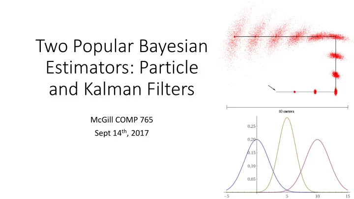
Consider distributions to each p(x| zi)

nly. Are these related to our answer?

SLIDE 10

10

Distributions

Wanted: samples distributed according to p(x| z1, z2, z3)

SLIDE 11

This is Easy!

We can draw samples from p(x|zl) by adding noise to the detection parameters.

SLIDE 12

Importance Sampling

As seen, it is often easy to draw samples from one portion of our Bayes filter
Main trick: importance sampling, i.e. how to estimate properties/statistics of one distribution (f) given

samples from another distribution (g) For example, suppose we want to estimate the expected value of f given only samples from g.

SLIDE 13

Importance Sampling

As seen, it is often easy to draw samples from one portion of our Bayes filter
Main trick: importance sampling, i.e. how to estimate properties/statistics of one distribution (f) given

samples from another distribution (g)

SLIDE 14

Importance Sampling

As seen, it is often easy to draw samples from one portion of our Bayes filter
Main trick: importance sampling, i.e. how to estimate properties/statistics of one distribution (f) given

samples from another distribution (g)

Weights describe the mismatch between the two distributions, i.e. how to reweigh samples to

btain statistics of f from

samples of g

SLIDE 15

Importance Sampling for Robocup

) ,..., , ( ) ( ) | ( ) ,..., , | ( : f

n

distributi Target

2 1 2 1 n k k n

z z z p x p x z p z z z x p



 ) ( ) ( ) | ( ) | ( : g

n

distributi Sampling

l l l

z p x p x z p z x p  ) ,..., , ( ) | ( ) ( ) | ( ) ,..., , | ( : w weights Importance

2 1 2 1 n l k k l l n

z z z p x z p z p z x p z z z x p g f





 

SLIDE 16

Importance Sampling

Weighted samples After resampling

Here are all of our p(x|zi) samples, now with w attached (not shown). If we re-draw from these samples, weighted by w, we get…

SLIDE 17

Importance Sampling for Bayes Filter

What is are the proposal distribution and weighting computations?

Recall: weighting to remove sample bias

Want posterior belief after update Sample from propagation, before update

SLIDE 18

Importance Sampling for Bayes Filter

What is are the proposal distribution and weighting computations?

This algorithm is known as a particle filter. Want posterior belief after update Sample from propagation, before update

SLIDE 19

Particle Filter Algorithm

Actual observation and control received

SLIDE 20

Particle Filter Algorithm

Particle propagation/prediction: noise needs to be added in order to make particles differentiate from each other. If propagation is deterministic then particles are going to collapse to a single particle after a few resampling steps.

SLIDE 21

Particle Filter Algorithm

Weight computation as measurement likelihood. For each particle we compute the probability of the actual observation given the state is at that particle.

SLIDE 22

Particle Filter Algorithm

Resampling step Note: particle deprivation heuristics are not shown here

SLIDE 23

Particle Filter Algorithm

Resampling: The particle locations now have a chance to adapt according to the weights. More likely particles persist, while unlikely choices are removed.

SLIDE 24

Examples: 1D Localization

SLIDE 25

Examples: 1D Localization

SLIDE 26

Resampling

Given: Set S of weighted samples.
Wanted : Random sample, where the probability of

drawing xi is given by wi.

Typically done n times with replacement to generate new

sample set S’.

SLIDE 27

w2 w3 w1 wn Wn-1

Resampling Carefully

w2 w3 w1 wn Wn-1

Roulette wheel
Binary search, n log n
Stochastic universal sampling
Systematic resampling
Linear time complexity
Easy to implement, low variance

SLIDE 28

1. Algorithm systematic_resampling(S,n):

2.

3. For

Generate cdf 4. 5. Initialize threshold

6. For

Draw samples … 7. While ( ) Skip until next threshold reached 8. 9. Insert 10. Increment threshold

11. Return S’

Resampling Algorithm

1 1

, ' w c S    n i  2 

i i i

w c c  

1

1 ], , ] ~

1 1





i n U u n j  1 

1 1  

  n u u

j j i j

c u 

 

   

1

, ' ' n x S S

i

1   i i

Also called stochastic universal sampling

SLIDE 29

Start

Particle Motion Model

SLIDE 30

Proximity Sensor Model Reminder

Laser sensor Sonar sensor

SLIDE 31

31

SLIDE 32

32

SLIDE 33

33

SLIDE 34

34

SLIDE 35

35

SLIDE 36

36

SLIDE 37

37

SLIDE 38

38

SLIDE 39

39

SLIDE 40

40

SLIDE 41

41

SLIDE 42

42

SLIDE 43

43

SLIDE 44

44

SLIDE 45

45

SLIDE 46

46

SLIDE 47

Particle Filter Summary

Very flexible tool as we get to make our choice of proposal

distributions (as long as we can properly compute importance weight)

Performance is guaranteed given infinite samples!
The particle cloud and its weights represent our distribution, but

making decisions can still be complex:

Act based on the most likely particle
Act using a weighted summation over particles
Act conservatively, accounting for the worst particle
In practice, the number of particles required to perform well scales

with the problem complexity and this can be hard to measure

SLIDE 48

Part 2: Kalman Filters

Intuition: track Bel(x) with a Gaussian distribution, simplifying

assumptions to ensure updates are all possible

Payoffs:
Continuous representation
Efficient computation
Uses:
Rocketry
Mobile devices
Drones
GPS
(the list is very long…)

SLIDE 49

Part 2: Kalman Filters

Intuition: track Bel(x) with a Gaussian distribution, simplifying

assumptions to ensure updates are all possible

Payoffs:
Continuous representation
Efficient computation
Uses:
Rocketry
Mobile devices
Drones
GPS
(the list is very long…)

SLIDE 50

Example: Landing on mars

SLIDE 51

Kalman Filter: an instance of Bayes’ Filter

Linear dynamics with Gaussian noise Linear observations with Gaussian noise Initial belief is Gaussian

Kalman Filter: Approach

SLIDE 52

Kalman Filter: assumptions

Two assumptions inherited from Bayes’ Filter
Linear dynamics and observation models
Initial belief is Gaussian
Noise variables and initial state

are jointly Gaussian and independent

Noise variables are independent and identically distributed
Noise variables are independent and identically distributed

SLIDE 53

Kalman Filter: why so many assumptions?

Two assumptions inherited from Bayes’ Filter
Linear dynamics and observation models
Initial belief is Gaussian
Noise variables and initial state

are jointly Gaussian and independent

Noise variables are independent and identically distributed
Noise variables are independent and identically distributed

Without linearity there is no closed-form solution for the posterior belief in the Bayes’ Filter. Recall that if X is Gaussian then Y=AX+b is also Gaussian. This is not true in general if Y=h(X). Also, we will see later that applying Bayes’ rule to a Gaussian prior and a Gaussian measurement likelihood results in a Gaussian posterior.

SLIDE 54

Kalman Filter: why so many assumptions?

Two assumptions inherited from Bayes’ Filter
Linear dynamics and observation models
Initial belief is Gaussian
Noise variables and initial state

are jointly Gaussian and independent

Noise variables are independent and identically distributed
Noise variables are independent and identically distributed

This results in the belief remaining Gaussian after each propagation and update step. This means that we only have to worry about how the mean and the covariance of the belief evolve recursively with each prediction step and update step  COOL!

SLIDE 55

Kalman Filter: why so many assumptions?

Two assumptions inherited from Bayes’ Filter
Linear dynamics and observation models
Initial belief is Gaussian
Noise variables and initial state

are jointly Gaussian and independent

Noise variables are independent and identically distributed
Noise variables are independent and identically distributed

This makes the recursive updates of the mean and covariance much simpler.

SLIDE 56

Kalman Filter: an instance of Bayes’ Filter

Assumptions guarantee that if the prior belief before the prediction step is Gaussian then the prior belief after the prediction step will be Gaussian and the posterior belief (after the update step) will be Gaussian.

SLIDE 57

Kalman Filter: an instance of Bayes’ Filter

So, under the Kalman Filter assumptions we get Belief after prediction step (to simplify notation) Notation: estimate at time t given history of observations and controls up to time t-1

SLIDE 58

Kalman Filter: an instance of Bayes’ Filter

So, under the Kalman Filter assumptions we get Two main questions: 1. How to get prediction mean and covariance from prior mean and covariance?

2. How to get posterior mean and covariance from

prediction mean and covariance? These questions were answered in the 1960s. The resulting algorithm was used in the Apollo missions to the moon, and in almost every system in which there is a noisy sensor involved  COOL!

SLIDE 59

Kalman Filter with 1D state

Let’s start with the update step recursion. Here’s an example:

Suppose your measurement model is with Suppose your first noisy measurement is Suppose your belief after the prediction step is Q: What is the mean and covariance of ?

SLIDE 60

Kalman Filter with 1D state: the update step

From Bayes’ Filter we get so

SLIDE 61

Kalman Filter with 1D state: the update step

From Bayes’ Filter we get so

Prediction residual/error between actual observation and expected

bservation.

You expected the measured mean to be 0, according to your prediction prior, but you actually observed 5. The smaller this prediction error is the better your estimate will be, or the better it will agree with the measurements.

SLIDE 62

Kalman Filter with 1D state: the update step

From Bayes’ Filter we get so

Kalman Gain: specifies how much effect will the measurement have in the posterior, compared to the prediction prior. Which one do you trust more, your prior ,

r your measurement ?

SLIDE 63

Kalman Filter with 1D state: the update step

From Bayes’ Filter we get so

The measurement is more confident (lower variance) than the prior, so the posterior mean is going to be closer to 5 than to 0.

SLIDE 64

Kalman Filter with 1D state: the update step

From Bayes’ Filter we get so

No matter what happens, the variance of the posterior is going to be reduced. I.e. new measurement increases confidence no matter how noisy it is.

SLIDE 65

Kalman Filter with 1D state: the update step

From Bayes’ Filter we get so

In fact you can write this as so and I.e. the posterior is more confident than both the prior and the measurement.

SLIDE 66

Kalman Filter with 1D state: the update step

From Bayes’ Filter we get so In this example:

SLIDE 67

Kalman Filter with 1D state: the update step

Another example:

SLIDE 68

Kalman Filter with 1D state: the update step

Take-home message: new observations, no matter how noisy, always reduce uncertainty in the posterior. The mean of the posterior, on the other hand,

nly changes when there is a nonzero prediction residual.

SLIDE 69