Groundwater modelling of the Ruamahanga Valley: USGS MODFLOW MT3D - - PowerPoint PPT Presentation

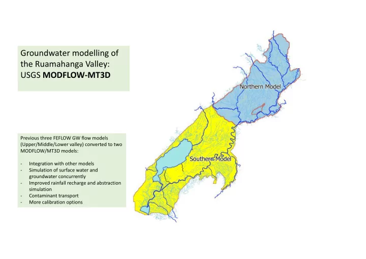
Groundwater modelling of the Ruamahanga Valley: USGS MODFLOW‐MT3D

Previous three FEFLOW GW flow models (Upper/Middle/Lower valley) converted to two MODFLOW/MT3D models: ‐ Integration with other models ‐ Simulation of surface water and groundwater concurrently ‐ Improved rainfall recharge and abstraction simulation ‐ Contaminant transport ‐ More calibration options

Groundwater Model Inputs & Assumptions

• Input 1: Physical structure: geology, layers, faults etc (FEFLOW)
• Input 2: Rivers/streams/springs (TOPNET / Mike11)
• Input 3: Rainfall recharge (IRRICALC)
• Input 4: Groundwater and surface water abstraction (IRRICALC)
• Input 5: Aquifer properties
• Input 6: Nutrient loadings (Overseer ‐ MPI / Jacobs)

Input 1: Geology and structure – physical model set up

• Complex geology. Conceptualisations developed for the Feflow models – robust

work based upon best current levels of understanding using best expertise available.

• Assumptions – there are numerous assumptions and simplifications in the

geological conceptualisations due to the highly complex and heterogeneous geological environment. This is unavoidable.

• Assumptions tested during the Feflow calibrations – the groundwater system

behaves as a single leaky system. The groundwater model probably least sensitive to assumptions made for Input 1.

• A highly interconnected groundwater system – which has strong connectivity to

surface water = basis for conjunctive sw/gw allocation management approach

Input 1: Geology/physical system structure

Input 2: Rivers/streams/springs – physical model set up

• Modflow’s SFR module (Stream Flow Routing) is a fundamental modelling component which

simulates channel flow and the interaction between surface water and groundwater.

• TOPNET feeds water into the SFR segments where rivers/streams enter the plains
• Surface water courses set up using GWRC bed survey and river cross‐section data (MIKE 11).
• SFR also simulates contaminant transport between groundwater and surface water.
• A big improvement over Feflow with regards its flexibility to integrate with other models.
• SFR handles inputs from overland flow/runoff, surface water abstractions (provided by

Irricalc), diversions to water races.

• Assumptions: Few flow monitoring sites on the plains for calibration; quite a few synthetic

flow sites based upon calculated relationships. Spatial resolution ‐ SFR set up using segments

• f about 2km length for major rivers – water balances therefore lumped for each segment.

SFR segments – Northern Model

(showing Topnet inputs at model boundary and water race injection nodes)

SFR segments – Southern Model

(also showing water race injection nodes)

Inputs 3 and 4: Rainfall recharge and irrigation demand (IRRICALC)

• Rainfall recharge externally calculated using a soil moisture balance model (IRRICALC). Similar methodology

to the previous feflow models although Irricalc is a more integrated soil water balance model which incorporates irrigation water demand and runoff.

• Irricalc requires input data: climate (rainfall and potential evapotranspiration), crop (crop factors, rooting

depths) and soil (soil water holding capacity) data. Provided by NIWA and Landcare Research.

• Recharge has been calculated using the same 500m grid and distributed input daily data rainfall and PET

series as used in the previous Feflow models (1992 to present).

• Irricalc has been used to model historic irrigation abstraction rates based upon crop water demand. These

demands have been incorporated into the model calibration (either as surface water or groundwater abstractions)

• Assumptions: Recharge calculated using soil moisture balance models assumes a free‐draining soil;

recharge is applied directly to the water table/aquifer and does not take into account unsaturated zone properties/lags or short‐circuits; irrigation demands assume certain irrigation practices/rules and land use; water is always available for irrigation at the rate required; assumptions concerning irrigation returns; assumptions concerning partitioning of runoff/interflow and groundwater recharge.

Irricalc recharge

Input 5: Aquifer properties (hydraulic conductivity and storage)

• Aquifer properties are based upon the previous Feflow models – which relied upon field‐measured

transmissivity/storage data (starting values in MODFLOW – will be refined during calibration).

• Model values are restricted to field‐measured ranges (pumping tests).
• Model calibration allows for a more distributed/heterogeneous distribution of parameters – derived

through the calibration process.

• Assumptions – areas where no data exist – but nature of geology provides a good guide. Natural system is

highly heterogeneous so simplifications need to be made: model parameter estimation and uncertainty analysis will interrogate assumptions in terms of their effect on model predictive reliability.

Groundwater Model Outputs & Assumptions

• Output 1: Groundwater levels
• Output 2: Stream flows
• Output 3: Stream – groundwater fluxes
• Output 4: Nitrate concentrations

Model calibration is currently being revised due to new TOPNET and Nitrate model input files supplied.

Assumptions: Groundwater levels

• Weekly stress periods
• 5 model layers in the north
• 8 model layers in the south
• Pilot point parameters x original Feflow

parameter zones

• Irricalc estimated recharge, abstraction, and

quickflow

• Topnet estimated inflows to model

Output 1: Groundwater levels

Output 2: Stream flows Assumptions: Stream flows

• Weekly stream flows used as calibration

targets

• Irricalc estimated recharge, abstraction, and

quickflow

• Topnet estimated inflows to model

Output 2: Stream flows

Output 2: Stream flows

Output 3: Stream – groundwater fluxes

Output 4: Nitrate concentrations Assumptions: Groundwater concentrations

• Annual average nitrate input into model from

Overseer

• Average nitrate concentration in surface water

ways as input into model (will iterate with Esource for final model version)

• 5 model layers in the north
• 8 model layers in the south
• Calibrated to average nitrate concentrations in

groundwater (monitoring period dependant) Pending new nitrate inputs…

Used 0.5 for initial condition