Graph Traversal Graph Traversal with DFS/BFS One of the most - PowerPoint PPT Presentation

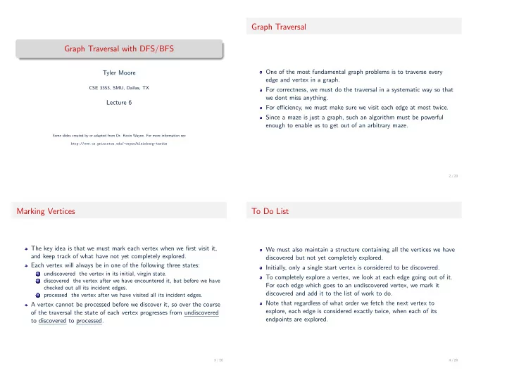
Graph Traversal Graph Traversal with DFS/BFS One of the most fundamental graph problems is to traverse every Tyler Moore edge and vertex in a graph. CSE 3353, SMU, Dallas, TX For correctness, we must do the traversal in a systematic way so that we dont miss anything. Lecture 6 For e ffi ciency, we must make sure we visit each edge at most twice. Since a maze is just a graph, such an algorithm must be powerful enough to enable us to get out of an arbitrary maze. Some slides created by or adapted from Dr. Kevin Wayne. For more information see http://www.cs.princeton.edu/~wayne/kleinberg-tardos 2 / 20 Marking Vertices To Do List The key idea is that we must mark each vertex when we fi rst visit it, We must also maintain a structure containing all the vertices we have and keep track of what have not yet completely explored. discovered but not yet completely explored. Each vertex will always be in one of the following three states: Initially, only a single start vertex is considered to be discovered. undiscovered the vertex in its initial, virgin state. 1 To completely explore a vertex, we look at each edge going out of it. discovered the vertex after we have encountered it, but before we have 2 For each edge which goes to an undiscovered vertex, we mark it checked out all its incident edges. discovered and add it to the list of work to do. processed the vertex after we have visited all its incident edges. 3 Note that regardless of what order we fetch the next vertex to A vertex cannot be processed before we discover it, so over the course explore, each edge is considered exactly twice, when each of its of the traversal the state of each vertex progresses from undiscovered endpoints are explored. to discovered to processed. 3 / 20 4 / 20

In what order should we process vertices? Depth-First Traversal Undirected Graph Depth-First Search Tree a 1 7 1 First-in- fi rst-out: if we use a queue to process discovered vertices, we b b b b f use breadth- fi rst search c c c 2 2 Last-in- fi rst-out: if we use a stack to process discovered vertices, we use depth- fi rst search a a a c 6 d d d 5 3 e e e f f f d 4 a c e Discovered: b d f e c a e Processed: d b f 5 / 20 6 / 20 Recursive Depth-First Traversal Code Iterative Depth-First Traversal Code i t e r d f s (G, s ) : def S , Q = s e t ( ) , [ ] # V i si te d − s e t and queue r e c d f s (G, s , S=None ) : def Q. append ( s ) # We plan on v i s i t i n g s i f S i s None : S = s e t () # I n i t i a l i z e the h i s t o r y while Q: # Planned nodes l e f t ? S . add ( s ) # We ’ ve v i s i t e d s u = Q. pop () # Get one for u in G[ s ] : # Explore neighbors i f u in S : continue # Already v i s i t e d ? Skip i t i f u in S : continue # Already v i s i t e d : Skip S . add (u) # We ’ ve v i s i t e d i t now r e c d f s (G, u , S) # New : Explore r e c u r s i v e l y Q. extend (G[ u ] ) # Schedule a l l neighbors y i e l d u # Report u as v i s i t e d > r e c d f s t e s t e d (G, 0) > > [0 , 1 , 2 , 3 , 4 , 5 , 6 , 7] > l i s t ( i t e r d f s (G, 0)) > > [0 , 5 , 7 , 6 , 2 , 3 , 4 , 1] 7 / 20 8 / 20

What does the yield command do? Breadth-First Traversal Undirected Graph Breadth-First Search Tree When you execute a function, it normally return s values a b b b Generators only execute code when iterated 1 3 c c c 2 Useful when you don’t need to keep the list of values you loop over 5 a a a e b f Especially helpful when the object you’re iterating over is very large, and you don’t want to keep the entire object in memory d d d 4 6 7 Nice explanation on Stack Over fl ow: http://stackoverflow.com/ e e e c f f f d questions/231767/the-python-yield-keyword-explained a e c b f d Discovered: a e c b f d Processed: 9 / 20 10 / 20 Breadth-First Traversal Code Correctness of Graph Traversal from c o l l e c t i o n s import deque i t e r b f s (G, s , S = None ) : def Every edge and vertex in the connected component is eventually S , Q = s e t ( ) , deque () # V i s i ted − s e t and queue visited. Why? Q. append ( s ) # We plan on v i s i t i n g s Suppose it’s not correct, ie. there exists an unvisited vertex A whose while Q: # Planned nodes l e f t ? neighbor B was visited. u = Q. p o p l e f t () # Get one When B was visited, each of its neighbors was added to the list to be u in S : i f continue # Already v i s i t e d ? Skip i t processed. Since A is a neighbor of B , it must be visited before the S . add (u) # We ’ ve v i s i t e d i t now algorithm completes. Q. extend (G[ u ] ) # Schedule a l l neighbors y i e l d u # Report u as v i s i t e d 11 / 20 12 / 20

Preorder vs. postorder processing Preorder and postorder processing with BFS def b f s p p (G, s , S = None ) : S , Q = s e t ( ) , deque () # V i s i t e d − s e t and queue Q. append ( s ) # We plan on v i s i t i n g s while Q: # Planned nodes l e f t ? u = Q. p o p l e f t () # Get one i f u i n S : continue # Already v i s i t e d ? Skip i t p r i n t ’ pre ’+u # p r e o r d e r p r o c e s s i n g − − aka p r o c e s s v e r t e x e a r l y (ADM) Many useful algorithms are built on top of BFS or DFS traversal S . add ( u ) # We ’ ve v i s i t e d i t now Q. extend (G[ u ] ) # Schedule a l l n e i g h b o r s Frequently, extra code is added either immediately before a node is y i e l d u # Report u as v i s i t e d processed (preorder processing) or after a node is processed p r i n t ’ − − post ’+u # p o s t o r d e r p r o c e s s i n g − − aka p r o c e s s v e r t e x l a t e − − − − (postorder processing) > l i s t ( b f s p p (N, ’ a ’ ) ) > > pre a − post a − − − − − pre b − post b − − − − − pre e − post e − − − − − pre f − post f − − − − − pre c − post c − − − − − pre d − post d − − − − − [ ’ a ’ , ’ b ’ , ’ e ’ , ’ f ’ , ’ c ’ , ’ d ’ ] 13 / 20 14 / 20 Preorder and postorder processing with DFS DFS Trees: all descendants of a node u are processed after u is discovered but before u is processed def r e c d f s p p (G, s , S=None ) : i f S i s None : S = s e t () # I n i t i a l i z e the h i s t o r y Undirected Graph Depth-First Search Tree S . add ( s ) # We ’ ve v i s i t e d s p r i n t ’ pre : ’+s # p r i n t node − − p r e o r d e r p r o c e s s i n g a u i n G[ s ] : # Explore n e i g h b o r s f o r 1 i f u i n S : continue # Already v i s i t e d : Skip 1 0 r e c d f s p p (G, u , S) # New : Explore r e c u r s i v e l y p r i n t ’ − − post : ’+s # p r i n t node − − p o s t o r d e r p r o c e s s i n g − − − − b b b b f S return c c c 2 > l i s t ( r e c d f s p p (N, ’ a ’ )) > > pre : a a a a c pre : b 6 pre : c pre : d pre : e d d d 5 3 − post : e − − − − − − post : d − − − − − e e e f f f d − post : c − − − − − − post : b − − − − − pre : f 4 − post : f − − − − − a c e Discovered: b d f − post : a − − − − − [ ’ a ’ , ’ c ’ , ’ b ’ , ’ e ’ , ’ d ’ , ’ f ’ ] e c a e Processed: d b f 15 / 20 16 / 20

How can we tell if one node is a descendant of another? Code for depth- fi rst timestamps dfs (G, s , d , f , S=None , t =0): def i f S i s None : S = s e t () # I n i t i a l i z e the h i s t o r y d [ s ] = t ; t += 1 # Set d i s c o v e r time S . add ( s ) # We ’ ve v i s i t e d s Answer: with depth- fi rst timestamps! for u in G[ s ] : # Explore neighbors After we create a graph in a depth- fi rst traversal, it would be nice to i f u in S : continue # Already v i s i t e d . Skip be able to verify if node A is encountered before node B , etc. t = dfs (G, u , d , f , S , t ) # Recurse ; update We add one timestamp for when a node is discovered (during preorder f [ s ] = t ; t += 1 # Set f i n i s h time processing) and another timestamp for when a node is processed return t # Return timestamp (during postorder processing) > > > f= {} > d= {} > > > d f s (N, ’ a ’ ,d , f ) > > 12 > d > > { ’ a ’ : 0 , ’ c ’ : 2 , ’ b ’ : 1 , ’ e ’ : 4 , ’ d ’ : 3 , ’ f ’ : 9 } > f > > { ’ a ’ : 11 , ’ c ’ : 7 , ’ b ’ : 8 , ’ e ’ : 5 , ’ d ’ : 6 , ’ f ’ : 10 } 17 / 20 18 / 20 Edge cases for DFS/BFS traversal Edge classi fi cation Tree edges Forward edge a a 1 Edge ( u , v ) is a tree edge if v was fi rst discovered by exploring edge c c b b ( u , v ). 2 Edge ( u , v ) is a back edge if vertex u is connected to an ancestor v . e e d d 3 Edge ( u , v ) is a forward edge if vertex u is connected to a descendant v . Back edge Cross edges 4 All other edges are cross edges a a c c b b e e d d 19 / 20 20 / 20