
SLIDE 1
GIT Graphs
- A. Ada, K. Sutner
Carnegie Mellon University Spring 2018
Outline
2
1
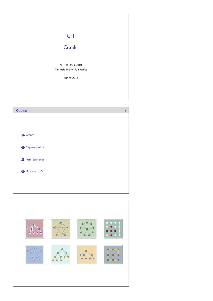
Graphs
2
Representation
3
Path Existence
4
GIT Graphs A. Ada, K. Sutner Carnegie Mellon University Spring - - PDF document
GIT Graphs A. Ada, K. Sutner Carnegie Mellon University Spring 2018 Outline 2 Graphs 1 Representation 2 Path Existence 3 BFS and DFS 4 Ancient History 4 A quote from a famous mathematician (homotopy theory): Combinatorics (read:
2
1
2
3
4
4
5
6
7
8
9
10
2
12
13
14
15
16
17
18
19
20
21
22
23
1
2 3
4 5
6
24
25
26
1 2 5 8 3 6 9 4 7 10
1 2 5 8 3 6 9 10 7 4
27
1 2 5 8 3 6 9 10 7 4
28
29
30
1
2 3
4 5
6
7
8
9
31
32
1
2 3
4
5 6
7
8
9
10
11
12
13
33
3
35
36
37
38
k A(i, k) · B(k, j) (standard Boolean algebra).
39
40
41
42
43
44
45
4
47
48
1 2
3 4
5
6 7
8
49
50
51
1 2
3 4
5
6
7
8 9
10
52
53
1 2
3
4
5
6 7
8
9
10
11
12
13
14
15
54
1
2
3
4
5
6
7
55
1
2
3
4
5 6
7
8
9
10
11
12
13
14
56
57 1 2 4 3 5 7 6 8 10 9
58
1
2
3
4
5
1
2 3
4 5
59 1 2 4 3 5 7 6 8 10 9
60
61
62
63 1 2 4 3 5 7 6 8 10 9
64
65
66