Geometry of Gaussoids Bernd Sturmfels MPI Leipzig and UC Berkeley p - - PowerPoint PPT Presentation

Geometry of Gaussoids

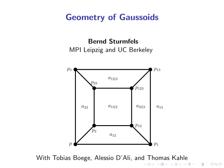
Bernd Sturmfels MPI Leipzig and UC Berkeley

p p1 p13 p3 p2 p12 p123 p23 a23 a23|1 a13 a13|2 a12 a12|3

With Tobias Boege, Alessio D’Ali, and Thomas Kahle

Matroids

12 34 24 14 23 13

A matroid is a combinatorial structure that encodes independence in linear algebra and geometry. The basis axioms reflect the ideal

• f homogeneous relations among all minors of a rectangular matrix

1

• 1
• =

1 0 −p23 −p24 1 p13 p14

• A matroid is an assignment of 0 or ⋆ to these minors so that

the quadratic Pl¨ ucker relations have a chance of vanishing: p12p34 − p13p24 + p14p23 = 0. We also like oriented matroids, positroids and valuated matroids.

Gaussoids

A gaussoid is a combinatorial structure that encodes independence in probability and statistics. The gaussoid axioms reflect the ideal

• f homogeneous relations among the principal and almost-principal

minors of a symmetric matrix 1

• 1
• =

1 p1 a12 1 a12 p2

• A gaussoid is an assignment of 0 or ⋆ to these minors so that

the quadratic Pl¨ ucker relations have a chance of vanishing: p · p12 − p1 · p2 + a2

12 = 0.

Ditto: oriented gaussoids, positive gaussoids, valuated gaussoids.

The gaussoid axioms were introduced in [R. Lnˇ eniˇ cka and F. Mat´ uˇ s: On Gaussian conditional independence structures, Kybernetika (2007)]

Principal and almost-principal minors

A symmetric n × n-matrix Σ has 2n principal minors pI

• ne for each subset I of [n] = {1, 2, . . . , n}.

The matrix Σ has 2n−2n

2

• almost-principal minors aij|K.

This is the subdeterminant of Σ with row indices {i} ∪ K and column indices {j} ∪ K, where i, j ∈ [n] and K ⊆ [n]\{i, j}.

Principal minors are in bijection with the vertices of the n-cube. Almost-principal minors are in bijection with the 2-faces of the n-cube.

Σ =   p1 a12 a13 a12 p2 a23 a13 a23 p3  

p p1 p13 p3 p2 p12 p123 p23 a23 a23|1 a13 a13|2 a12 a12|3

Why Gauss?

If Σ is positive definite then it is the covariance matrix of a Gaussian distribution on Rn. In statistics: pI > 0 for all I ⊆ [n]. Study n random variables X1, X2, . . . , Xn, with the aim of learning how they are related. (Yes, data science) Almost-principal minors aij|K measure partial correlations. We have aij|K = 0 if and only if Xi and Xj are conditionally independent given XK. The inequalities aij|K > 0 and aij|K < 0 indicate whether conditional correlation is positive or negative.

Ideals, Varieties, ...

Write Jn for the homogeneous prime ideal of relations among the principal and almost-principal minors of a symmetric n × n-matrix. It lives in a polynomial ring R[p, a] with N = 2n + 2n−2n

2

• unknowns, and defines an irreducible subvariety of PN−1.

Proposition

The projective variety V (Jn) is a coordinate projection of the Lagrangian Grassmannian. They share dimension and degree: dim(V (Jn)) = n+1

2

• degree(V (Jn)) =

n+1

2

• !

1n · 3n−1 · 5n−2 · · · (2n − 1)1 . The elimination ideal Jn ∩ R[p] was studied by Holtz-St and

• Oeding. They found hyperdeterminantal relations of degree 4.

3-cube

The ideal J3 is generated by 21 quadrics. There are 9 quadrics associated with the facets of the 3-cube: S200   (2, 0, 0) a2

23 + pp23 − p2p3

(0, 0, 0) 2a23a23|1 + pp123 + p1p23 − p2p13 − p12p3 (−2, 0, 0) a2

23|1 + p1p123 − p12p13

 

.... and two other such weight components

There are 12 trinomials associated with the edge of the 3-cube: S110     (1, 1, 0) a13a23 + a12|3p − a12p3 (1, −1, 0) a13|2a23 + a12|3p2 − a12p23 (−1, 1, 0) a13a23|1 + a12|3p1 − a12p13 (−1, −1, 0) a13|2a23|1 + a12|3p12 − a12p123    

.... and two other such weight components

The variety V (J3) is the Lagrangian Grassmannian in P13, which has dimension 6 and degree 16. It is arithmetically Gorenstein. Intersections with subspaces P8 are canonical curves of genus 9.

3-cube

Of most interest are the 12 edge trinomials: p1a23 − pa23|1 − a12a13 p2a13 − pa13|2 − a12a23 p3a12 − pa12|3 − a23a13 p12a13 − p1a13|2 − a12a23|1 p12a23 − p2a23|1 − a12a13|2 p13a12 − p1a12|3 − a13a23|1 p13a23 − p3a23|1 − a13a12|3 p23a12 − p2a12|3 − a23a13|2 p23a13 − p3a13|2 − a23a12|3 p123a12 − p12a12|3 − a23|1a13|2 p123a13 − p13a13|2 − a23|1a12|3 p123a23 − p23a23|1 − a12|3a13|2

p p1 p13 p3 p2 p12 p123 p23 a23 a23|1 a13 a13|2 a12 a12|3

Gaussoid Axioms

Let A be the set of n

2

• 2n−2 symbols aij|K. Following Lnˇ

eniˇ cka and Mat´ uˇ s, a subset G of A is a gaussoid on [n] if it satisfies:

• 1. {aij|L, aik|jL} ⊂ G implies {aik|L, aij|kL} ⊂ G,
• 2. {aij|kL, aik|jL} ⊂ G implies {aij|L, aik|L} ⊂ G,
• 3. {aij|L, aik|L} ⊂ G implies {aij|kL, aik|jL} ⊂ G,
• 4. {aij|L, aij|kL} ⊂ G implies
• aik|L ∈ G or ajk|L ∈ G
• .

These axioms are known as

• 1. semigraphoid, 2. intersection,
• 3. converse to intersection, 4. weak transitivity.

Gaussoid Axioms

Let A be the set of n

2

• 2n−2 symbols aij|K. Following Lnˇ

eniˇ cka and Mat´ uˇ s, a subset G of A is a gaussoid on [n] if it satisfies:

• 1. {aij|L, aik|jL} ⊂ G implies {aik|L, aij|kL} ⊂ G,
• 2. {aij|kL, aik|jL} ⊂ G implies {aij|L, aik|L} ⊂ G,
• 3. {aij|L, aik|L} ⊂ G implies {aij|kL, aik|jL} ⊂ G,
• 4. {aij|L, aij|kL} ⊂ G implies
• aik|L ∈ G or ajk|L ∈ G
• .

These axioms are known as

• 1. semigraphoid, 2. intersection,
• 3. converse to intersection, 4. weak transitivity.

Theorem

The following are equivalent for a set G of 2-faces of the n-cube: (a) G is a gaussoid, i.e. the four axioms above are satisfied for G. (b) G is compatible with the quadratic edge trinomials in Jn.

Duality and Minors

Let G be any gaussoid on [n]. The dual of G is G∗ =

• aij|L : aij|K ∈ G and L = [n]\({i, j} ∪ K)
• .

Fix an element u ∈ [n]. The marginalization equals G\u =

• aij|K ∈ G : u ∈ {i, j} ∪ K
• .

The conditioning equals G/u =

• aij|K\{u} : aij|K ∈ G and u ∈ K
• .

Think of operations on sets of 2-faces of the n-cube.

Proposition

If G is a gaussoid on [n], and u ∈ [n], then G∗, G\u and G/u are gaussoids on [n]\{u}. The following duality relation holds:

• G\u

∗ = G∗/u and

• G/u

∗ = G∗\u. If G is realizable (with Σ positive definite) then so are G∗, G\u, G/u.

A Pinch of Representation Theory

Fix the Lie group G = (SL2(C))n. Write Vi ≃ C2 for the defining representation of the i-th factor. The irreducible G-modules are Sd1d2···dn =

n

• i=1

Symdi(Vi),

Proposition

G acts on the space Wpr spanned by the principal minors and the spaces W ij

ap spanned by almost-principal minors. As G-modules,

Wpr ≃ ⊗n

i=1Vi

and W ij

ap ≃ ⊗k∈[n]\{i,j}Vk

for 1 ≤ i < j ≤ n.

This defines the G-action and Zn-grading on our polynomial ring C[p, a]. The formal character of C[p, a]1 = Wpr ⊕

i,jW ij ap is the sum of weights:

n

i=1(xi + x−1 i

) +

1≤i<j≤n

• k∈[n]\{i,j}(xk + x−1

k )

Commutative Algebra

The number of linearly independent quadrics in the ideal Jn equals

3n−2 n 2

• + 2

n−3

• k=0

3k(n − k)(n − k − 1) n k

• + 2

⌊ n

2 ⌋

• k=2

k3n−2k n 2k

• Derived via the lowering and raising operators in the Lie algebra g.

Conjecture

These quadrics generate Jn.

Proposition

The number of face trinomials and edge trinomials equals 2n−2 n 2

• + 12 · 2n−3

n 3

• = 2n−3n(n − 1)(2n − 3).

These trinomials generate the image of Jn in C[p, a±].

4-cube

p p1 p13 p3 p2 p12 p123 p23 a23 a23|1 a13 a13|2 a12 a12|3

There are 16 principal and 24 almost principal minors. They span C[p, a]1 = S1111 ⊕ S1100 ⊕ S1010 ⊕ S1001 ⊕ S0110 ⊕ S0101 ⊕ S0011.

The space of quadrics has dimension 820. As G-module, C[a, p]2 ≃ S2222 ⊕ S2211 ⊕ S2121 ⊕ S2112 ⊕ S1221 ⊕ S1212 ⊕ S1122 ⊕ 2S2200 ⊕ 2S2020 ⊕2S2002 ⊕ 2S0220 ⊕ 2S0202 ⊕ 2S0022 ⊕ 2S2110 ⊕ 2S2101 ⊕ 2S2011 ⊕ 2S1210 ⊕2S1201 ⊕ 2S0211 ⊕ 2S1120 ⊕ 2S1021 ⊕ 2S0121 ⊕ 2S1102 ⊕ 2S1012 ⊕ 2S0112 ⊕3S1111 ⊕ 3S1100 ⊕ 3S1010 ⊕ 3S1001 ⊕ 3S0110 ⊕ 3S0101 ⊕ 3S0011 ⊕ 7S0000. The 226-dimensional submodule (J4)2 of quadrics in our ideal equals S2200 ⊕ S2020 ⊕ S2002 ⊕ S0220 ⊕ S0202 ⊕ S0022 ⊕ S2110 ⊕ S2101 ⊕ S2011 ⊕S1210 ⊕ S1201 ⊕ S0211 ⊕ S1120 ⊕ S1021 ⊕ S0121 ⊕ S1102 ⊕ S1012 ⊕S0112 ⊕ S1100 ⊕ S1010 ⊕ S1001 ⊕ S0110 ⊕ S0101 ⊕ S0011 ⊕ 4S0000. Of these, 120 are trinomials: 96 edge trinomials and 24 face trinomials.

Enumeration of Gaussoids

Theorem

The number of gaussoids for n = 3, 4, 5 equals: n all gaussoids

• rbits for Sn

Z/2Z ⋊ Sn (Z/2Z)n ⋊ Sn 3 11 5 4 4 4 679 58 42 19 5 60, 212, 776 508, 817 254, 826 16, 981

For n = 3, all 11 gaussoids are realizable: {}, {a12}, {a13}, {a23}, {a12|3}, {a13|2}, {a23|1}, {a12, a12|3, a13, a13|2}, {a12, a12|3, a23, a23|1}, {a13, a13|2, a23, a23|1}, {a12, a12|3, a13, a13|2, a23, a23|1}.

Enumeration of Gaussoids

Theorem

The number of gaussoids for n = 3, 4, 5 equals: n all gaussoids

• rbits for Sn

Z/2Z ⋊ Sn (Z/2Z)n ⋊ Sn 3 11 5 4 4 4 679 58 42 19 5 60, 212, 776 508, 817 254, 826 16, 981

For n = 3, all 11 gaussoids are realizable: {}, {a12}, {a13}, {a23}, {a12|3}, {a13|2}, {a23|1}, {a12, a12|3, a13, a13|2}, {a12, a12|3, a23, a23|1}, {a13, a13|2, a23, a23|1}, {a12, a12|3, a13, a13|2, a23, a23|1}. For n = 4, five of the 42 gaussoid classes are non-realizable. For instance, G = {a12|3, a13|4, a14|2} is not realizable. Real Nullstellensatz certificate: a14

• a2

34p2p4p23 + a2 23a2 34p24 + p2 2p3p4p34

• − (a23a24a34 + p2p3p4)(a24p4a12|3 + a24a23a13|4 + p3p4a14|2) ∈ J4.

SAT Solvers

Current software for the satisfiability problem is very impressive, and useful for enumerating combinatorial structures like gaussoids. The input is a Boolean formula in conjunctive normal form (CNF). One can specify one of the following three output options:

◮ SAT: Is the formula satisfiable? ◮ #SAT: How many satisfying assignments are there? ◮ AllSAT: Enumerate all satisfying assignments.

We found the 60, 212, 776 gaussoids for n = 5 in about one hour using Thurley’s software bdd minisat all. The input was a SAT formulation of the gaussoid axioms using 1680 clauses in the CNF. We then analyzed the output with respect to the symmetry groups.

Oriented gaussoids

An oriented gaussoid is a map A → {0, ±1} such that, for each edge trinomial, after setting each pI to +1 and each aij|K to its image, the set of signs of terms is {0} or {−1, +1} or {−1, 0, +1}.

Analogous to oriented matroids.

A positive gaussoid is an assignment A → {0, +1} with the same compatibility requirement.

Analogous to positroids.

Oriented gaussoids

An oriented gaussoid is a map A → {0, ±1} such that, for each edge trinomial, after setting each pI to +1 and each aij|K to its image, the set of signs of terms is {0} or {−1, +1} or {−1, 0, +1}.

Analogous to oriented matroids.

A positive gaussoid is an assignment A → {0, +1} with the same compatibility requirement.

Analogous to positroids.

Example Let n = 3. Each singleton gaussoid, like G = {a12} or {a12|3} supports four oriented gaussoids, related by reorientation. We display these 24 = 6 × 4 oriented gaussoids by listing the six signs for A in the order a12, a13, a23, a12|3, a13|2, a23|1:

0 − − − − − 0 − + + −+ 0 + − + +− 0 + + − + + + 0 + + − + − 0 − − − − − 0 + − + + + 0 − + + − + − 0 + −+ − − 0 − −− − + 0 − ++ + + 0 + +− + − − 0 − − − − + 0 − + − + − 0 + − + + + 0 + + − − + − 0 + + − − + 0 − + + + + 0 + − + − − 0 − − + − − + 0 + + + + + 0 + − − + − 0 − − + − − 0

3-Cube and Beyond

Proposition

For n=3 there are 51 oriented gaussoids in seven symmetry classes. All are realizable. This includes 20 uniform gaussoids A → {±1}.

The following table exhibits the seven classes. The first column gives a covariance matrix Σ that realizes the first oriented gaussoid in the class: (p1,p2,p3, a12,a13,a23) Symmetry class of oriented gaussoids (2, 2, 2, 1, 1, 1) ++++++, +−−+−−, −−+−−+, −+−−+− (3, 5, 1, 1, 1, 2) +++−++, +−−−−−, −−++− +, . . . , −−+−−− (6, 9, 6, −1, −1, −7) −−−−−−, ++−++ −, −++−++, +−++−+ (4, 3, 3, 2, 2, 1) +++++0, ++++0+, . . . previous page (2, 2, 2, 0, −1, −1) 0−−−−−, 0−++−+, . . . previous page (3, 2, 2, 0, 0, 1) 00+00+, 00−00−, −00−00, . . . , 0+00+0 (1, 1, 1, 0, 0, 0) 000000

3-Cube and Beyond

Proposition

For n=3 there are 51 oriented gaussoids in seven symmetry classes. All are realizable. This includes 20 uniform gaussoids A → {±1}.

The following table exhibits the seven classes. The first column gives a covariance matrix Σ that realizes the first oriented gaussoid in the class: (p1,p2,p3, a12,a13,a23) Symmetry class of oriented gaussoids (2, 2, 2, 1, 1, 1) ++++++, +−−+−−, −−+−−+, −+−−+− (3, 5, 1, 1, 1, 2) +++−++, +−−−−−, −−++− +, . . . , −−+−−− (6, 9, 6, −1, −1, −7) −−−−−−, ++−++ −, −++−++, +−++−+ (4, 3, 3, 2, 2, 1) +++++0, ++++0+, . . . previous page (2, 2, 2, 0, −1, −1) 0−−−−−, 0−++−+, . . . previous page (3, 2, 2, 0, 0, 1) 00+00+, 00−00−, −00−00, . . . , 0+00+0 (1, 1, 1, 0, 0, 0) 000000

Theorem

The number of oriented gaussoids is 34,873 for n = 4, and it is 54936241913 for n = 5. Among these, 878349984 are uniform.

From Positroids to Statistics

Positroids are oriented matroids whose bases are positive. These are important in representation theory and algebraic combinatorics, and they have desirable topological properties. Positive gaussoids correspond to distributions that are of current interest in statistics:

S.Fallat, S.Lauritzen, K.Sadeghi, C.Uhler, N.Wermuth and P.Zwiernik: Total positivity in Markov structures, Annals of Statistics 45 (2017)

• F. Mohammadi, C. Uhler, C. Wang and J. Yu: Generalized permutohedra

from probabilistic graphical models, arXiv:1606.01814.

• S. Lauritzen, C. Uhler and P. Zwiernik: Maximum likelihood estimation

in Gaussian models under total positivity, arXiv:1702.04031.

From Positroids to Statistics

Positroids are oriented matroids whose bases are positive. These are important in representation theory and algebraic combinatorics, and they have desirable topological properties. Positive gaussoids correspond to distributions that are of current interest in statistics:

S.Fallat, S.Lauritzen, K.Sadeghi, C.Uhler, N.Wermuth and P.Zwiernik: Total positivity in Markov structures, Annals of Statistics 45 (2017)

• F. Mohammadi, C. Uhler, C. Wang and J. Yu: Generalized permutohedra

from probabilistic graphical models, arXiv:1606.01814.

• S. Lauritzen, C. Uhler and P. Zwiernik: Maximum likelihood estimation

in Gaussian models under total positivity, arXiv:1702.04031.

Ardila, Rinc´

• n and Williams (2017) proved a 1987 conjecture
• f Da Silva by showing that all positroids are realizable.

We derive the analogue for gaussoids: all positive gaussoids are realizable and their realization spaces are very nice.

Positive Gaussoids are Graphical

Every graph Γ = ([n], E) defines a gaussoid GΓ via CI statements that hold for the graphical model Γ. Here, aij|K lies in GΓ iff every path from i to j in Γ passes through K. Thus aij ∈ GΓ when i and j are disconnected in Γ, and aij

• [n]\{i,j} ∈ GΓ when {i, j} ∈ E.

Theorem

For n ≥ 2, there are precisely 2(n

2) positive gaussoids. All are

realizable from graphs as above. The space of covariance matrices Σ that realize GΓ is homeomorphic to a ball of dimension |E| + n.

◮ The concentration matrices Σ−1 are M-matrices with support Γ.

[S. Karlin and Y. Rinott: M-matrices as covariance matrices of multinormal distributions, Linear Algebra Appl. (1983)]

◮ Positive gaussoids satisfy the axiomatic requirements in [K. Sadeghi:

Faithfulness of probability distributions and graphs, arXiv:1701..]

Conclusion

Matroids are cool. And so are gaussoids. Positivity is crucial in algebraic combinatorics. And in statistics. On this journey, let the quadratic equations be your guide. Hitch a fast ride using SAT solvers and representation theory.

p1a23 − pa23|1 − a12a13, p2a13 − pa13|2 − a12a23, p3a12 − pa12|3 − a23a13, p12a13 − p1a13|2 − a12a23|1, p12a23 − p2a23|1 − a12a13|2, . . .

Conclusion

Matroids are cool. And so are gaussoids. Positivity is crucial in algebraic combinatorics. And in statistics. On this journey, let the quadratic equations be your guide. Hitch a fast ride using SAT solvers and representation theory.

p1a23 − pa23|1 − a12a13, p2a13 − pa13|2 − a12a23, p3a12 − pa12|3 − a23a13, p12a13 − p1a13|2 − a12a23|1, p12a23 − p2a23|1 − a12a13|2, . . .

p p1 p13 p3 p2 p12 p123 p23 a23 a23|1 a13 a13|2 a12 a12|3

Thank You

Stay tuned for valuated gaussoids via tropical Lagrangian Grassmannian.