General feedback system Relevant relations/transfer functions + v - - PowerPoint PPT Presentation

General feedback system

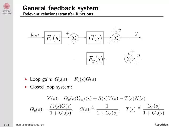
Relevant relations/transfer functions

yref y v n + + + + + −

G(s) Fy(s) Fr(s)

Σ Σ Σ

◮ Loop gain: Go(s) = Fy(s)G(s) ◮ Closed loop system:

Y (s) = Gc(s)Yref(s) + S(s)V (s) − T(s)N(s) Gc(s) = Fr(s)G(s) 1 + Go(s) , S(s) 1 1 + Go(s), T(s) Go(s) 1 + Go(s)

1 / 8 hans.rosth@it.uu.se Repetition

Bode plots

Frequency domain models

Example: Second order system G(s) = ω2 s2 + 2ζω0s + ω2 , poles in − ω0

• ζ ± i
• 1 − ζ2
• ω0 = distance from the origin, ζ = damping ratio.

10

−1

10 10

1

10

−2

10

−1

10 10

1

ω/ω0 Gain ζ=0.3 ζ=1 ζ=0.5 ζ=0.1 ζ=0.05 10

−1

10 10

1

−180 −150 −120 −90 −60 −30 ω/ω0 Phase ( o) ζ=0.3 ζ=1 ζ=0.5 ζ=0.1 ζ=0.05

◮ Small damping ratio, ζ ≪ 1 ⇒ resonance peak

Mp ≥ |G(iω0)| = 1 2ζ

2 / 8 hans.rosth@it.uu.se Repetition

The Nyquist criterion

Stability for feedback systems

Let γ be a semicircle with radius R → ∞. Go(s) maps γ onto γ′. Re Re Im Im γ γ′ R Go(s) The Nyquist criterion:

◮ If γ′ encircles -1 k times counter clockwise, the closed loop

system has k more poles in the RHP than Go(s) has.

◮ If γ′ encircles -1 k times clockwise, the closed loop system has

k fewer poles in the RHP than Go(s) has.

3 / 8 hans.rosth@it.uu.se Repetition

The step response

Typical time domain specifications

r Tr Ts yf 0.1yf 0.9yf Myf e∞ = r − yf time Tr = risetime (10%–90% of yf) Ts = settling time (within p%) M = overshoot (often in % of yf) e∞ = steady state error

4 / 8 hans.rosth@it.uu.se Repetition

Specifications on the Nyquist curve Go(iω)

Stability margins

Re Im ωc ωp ω = ωc ω = ωp ω ω

• 1

−i ϕm ϕm

1 Am 1 Am

−180◦ 1 arg Go |Go|

5 / 8 hans.rosth@it.uu.se Repetition

State space representations

Controller canonical form

The system with the transfer function G(s) = b1sn−1 + · · · + bn−1s + bn sn + a1sn−1 + · · · + an−1s + an can be represented by the controller canonical form:                        ˙ x =          −a1 −a2 · · · −an−1 −an 1 · · · 1 · · · . . . . . . ... . . . . . . · · · 1          x +          1 . . .          u y =

• b1

b2 · · · bn

• x

6 / 8 hans.rosth@it.uu.se Repetition

State space representations

Observer canonical form

The system with the transfer function G(s) = b1sn−1 + · · · + bn−1s + bn sn + a1sn−1 + · · · + an−1s + an can be represented by the observer canonical form:                        ˙ x =          −a1 1 · · · −a2 1 · · · . . . . . . . . . ... . . . −an−1 · · · 1 −an · · ·          x +          b1 b2 . . . bn−1 bn          u y =

• 1

· · ·

• x

7 / 8 hans.rosth@it.uu.se Repetition

State space representations

Solution of the state equation

The initial value problem ˙ x(t) = Ax(t) + Bu(t), x(t0) = x0, has the solution x(t) = eA(t−t0)x0 + t

t0

eA(t−τ)Bu(τ)dτ. The matrix exponential function: eAt

∞

• k=0

1 k!(At)k, L[eAt] = (sI − A)−1

8 / 8 hans.rosth@it.uu.se Repetition