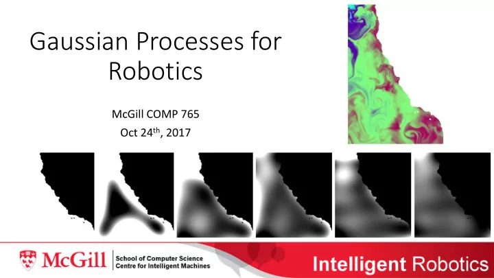
Gaussian Processes for Robotics McGill COMP 765 Oct 24 th , 2017 A - - PowerPoint PPT Presentation

Gaussian Processes for Robotics

McGill COMP 765 Oct 24th, 2017

A robot must learn

• Modeling the environment is sometimes an end goal:
• Space exploration
• Disaster recovery
• Environmental monitoring
• Other times, important sub-component of algorithms we know:
• x' = f(x,u)
• z = g(x)

Today: Learning for Robotics

• Which learned models are right for robotics?
• A look at some common robot learning problems
• Example problems that integrate learning:
• Planning to explore
• Active object recognition

Generative vs Discriminative Modeling

• Discriminative – how likely is the state given the observation, 𝑞(𝑦|𝑨):
• This can be used to directly answer some of the questions we care about,

such as localization

• It is not well suited for integration with other observations: 𝑞 𝑦 𝑨1, 𝑨2 ?
• Generative – how likely is the observation given the state, 𝑞(𝑨|𝑦):
• Does not directly provide the answer we desire, BUT
• A better fit as a sub-component of our techniques (recursive Bayesian filter,
• ptimal control, etc.)
• Provides the ability to sample, and a notion of prediction uncertainty

The robot learning problem

• From data observed so far, (x, z) pairs, learn a generative model that

can evaluate 𝑞(𝑨|𝑦𝑗) for unseen x that we encounter in the future

Gaussian Process Solution

• Gaussian Process (GP) is such a

generative model, also:

• Non-parametric
• Bayesian
• Kernel-based
• Core idea: use the input (x,y)

dataset directly to compute predictions of mean and variance at new points:

• As a function of the kernel

(intuitively: distance) between new point and training set

Gaussian Process Details

• Borrowed from excellent slides of Iain Murray at University of

Edinburgh

Review

• Gaussian processes are a non-parametric, non-linear estimator
• Learning and inference from data so far allows estimation of unknown

function values at query points along with prediction uncertainty

Today: How to choose useful samples?

• Depends on objective:
• Minimize uncertainty in estimated model
• Find the max or min
• Find areas of greatest change
• Reduce travel time
• Each of these can be accomplished by building on top
• f GP framework and have been used in applications

Measuring Uncertainty

• Each of our Bayesian models has a measure of its own uncertainty,

but this is sometimes complicated construction:

• Particle cloud
• Gaussian over robot pose for localization
• Gaussian over entire map and robot pose for SLAM
• Infinite dimensional Gaussian for GP
• How much knowledge is contained in each?

Measures of Uncertainty

• Variance (expected squared error)
• Entropy: H(p(x))
• KL Divergence from prior
• Maximum mean discrepancy
• Etc, etc
• There are many metrics. Each is good at

various things. For now, how to use them in practice?

Minimize Uncertainty

• Consider decision theoretic properties of a map (entropy, mutual

information):

• Search over potential robot locations
• Assume most likely measurement is received, or integrate uncertainty
• Select a single location, or path that minimizes entropy
• What is the analog for GPs?

Example from “Informative Planning with GP”

• Select new samples to visit

in the ocean that will maximize information gain

• Recall: entropy for Gaussian

distribution related to trace

• f covariance
• What is involved in

computing this entropy for

• ur GP model?

Computing GP Entropy

• GP co-variance is only a

function of sampled locations (for fixed hyper-parameters)

• Therefore, one can evaluate

the change in entropy that will

• ccur for sampling any location

without knowing the measurement

• So, it is easy to compute. But,

it ignores the measurements…. to be continued

Linking sampling locations

• “Informative Sampling…” paper chooses a fixed set of new points

using information gain criterion

• The set is constructed using dynamic programming
• Paths are constructed to join the points by solving a TSP
• Receding horizon: carry out part of the path, update the GP, re-plan

Acquisition functions

• One can formulate several different

criteria for balancing uncertainty and expected function values

• Iteratively select the maximum of this

function, sample the world, update GP

• Implicit assumption: acquisition function

is a trivial function of mean and variance

Commonly Used Acquisition Functions

• Probability of Improvement:
• Expected Improvement:
• Lower-confidence bound

Finding acquisition max

• What algorithm can we use to find the acquisition function’s maxima:
• It is non-linear
• We can compute local gradients, but the function will often be non-convex
• Evaluation of the acquisition function at a point requires performing GP

inference -> this can be expensive for large sets of high-dimensional data

Gradient-free Optimization

• This assumption allows regions to be eliminated from consideration

based on the values at their endpoints. The function values are constrained by a linear condition from each end:

• A famous approach using this assumption is Shubert’s 1972 algorithm

for minimization by successive decomposition into sub-regions

Shubert’s Algorithm

DIRECT: Dividing Rectangles

• For higher dimensional inputs, representing region boundary scales as

2n and computing optimal midpoint is costly

• Assuming knowledge of Lipschitz constant is also limiting
• DIRECT solves these problems:
• A clever mid-point sampling construction that allows regions to be

represented efficiently with a tree

• Optimizes over ALL possible Lipschitz constants [0,inf]
• Jones, Pertunnen and Stuckman. Lipschitzian Optimization Without the

Lipschitz Constant. Optimization Theory and Applications, 1993.

DIRECT Examples

DIRECT Pseudo-code

Potentially Optimal Regions

• Regions are of fixed size,

so discrete values of a-b

• Search over any possible

K means picking the lowest f(c) for each size

• We are simultaneously

searching globally and

• locally. Cool!
• Is the second condition

useful for unknown K?

Broader view

• Bayesian Optimization refers to the use of a GP, acquisition function

and sample-selection strategy to optimize a black-box function

• It has been used:
• To optimize the hyper-parameters of robotics, machine learning, and vision
• methods. It is still my person favorite here when you out-grow grid-search
• To win SAT solving competitions
• As a core component of some ML and robotics approaches (e.g., Juan’s recent

work on behavior adaptation)

• Alternatives to DIRECT exist:
• MCMC
• Variational methods

Back to Robotics: Additional constraints

• A robot cannot immediately sample a centre-point, but needs to

follow a fixed path

• It may not be able to follow the path precisely
• Many interesting algorithms result. More during Sandeep’s invited

talk!

Active Learning for Object Recognition

• Using GP as image classifier, we

can intelligently choose the examples for humans to label

• Example: Kapoor et al. Gaussian

Processes for Object Categorization, IJCV 2009.

• Several acquisition functions are

proposed (slight variations on those we’ve seen)

Active Learning Criteria

• Computed over unlabeled

images, using extracted features mapped through GP with “Pyramid Match Kernel”

• Observed labels are -1 or 1 to

indicate class membership

• Best performance achieved with

Uncertainty approach

Reducing Localization Uncertainty

• Assigned reading “A Bayesian Exploration-Exploitation Approach for

Optimal Online Sensing and Planning with a Visually Guided Mobile Robot”

• Searches for localization policies using Bayesian Optimization

Bayesian Exploration

GP Bayes Filter

• Recall: Recursive Bayesian filter for state estimation requires motion

and observation models. Traditionally, it is up to system designer to specify these, but they can be learned!

• [Ko and Fox, GP-BayesFilters: Bayesian filtering using Gaussian

process prediction and observation models Auton. Robot 2009]

GP EKF Experiments

• Blimp aero-dynamics are difficult to model, but data from motion

capture provides inputs for GPs

• Afterwards, learned model allows performance w/o mo-cap

Training data dependence

• The robot makes a left turn

when:

• It has suitable training data

(top)

• All left-turn data has been

removed (bottom)

• Predicted variance

increases, but tracking is still reasonable

Practical Robotics Extensions

• Heteroscedastic GP allows state-dependent noise models (we have

seen this last lecture)

• Sparse GPs allow for more efficient computation, at little cost in these

experiments

• How to best sparsify training data for robotics problems is an open question

Wrap-up and Review

• GP assumptions are a great fit for many robotics problems, and are

highly used in research today

• Combined with acquisition functions and global optimization, they

are a “black-box” optimizer that one can try nearly everywhere

• Primary limitation: computational complexity with training data
• More to come:
• We will see the use of Gaussian Processes in many different approaches for

direct exploration and the dynamics model embedded in RL learning methods