15.1 Last Lecture Want to solve a regression problem. confidence - - PDF document

CS/CNS/EE 253: Advanced Topics in Machine Learning Topic: Nonparametric learning #4: Gaussian Process Regression Lecturer: Andreas Krause Scribe: Tim Black Date: March 1, 2010

15.1 Last Lecture

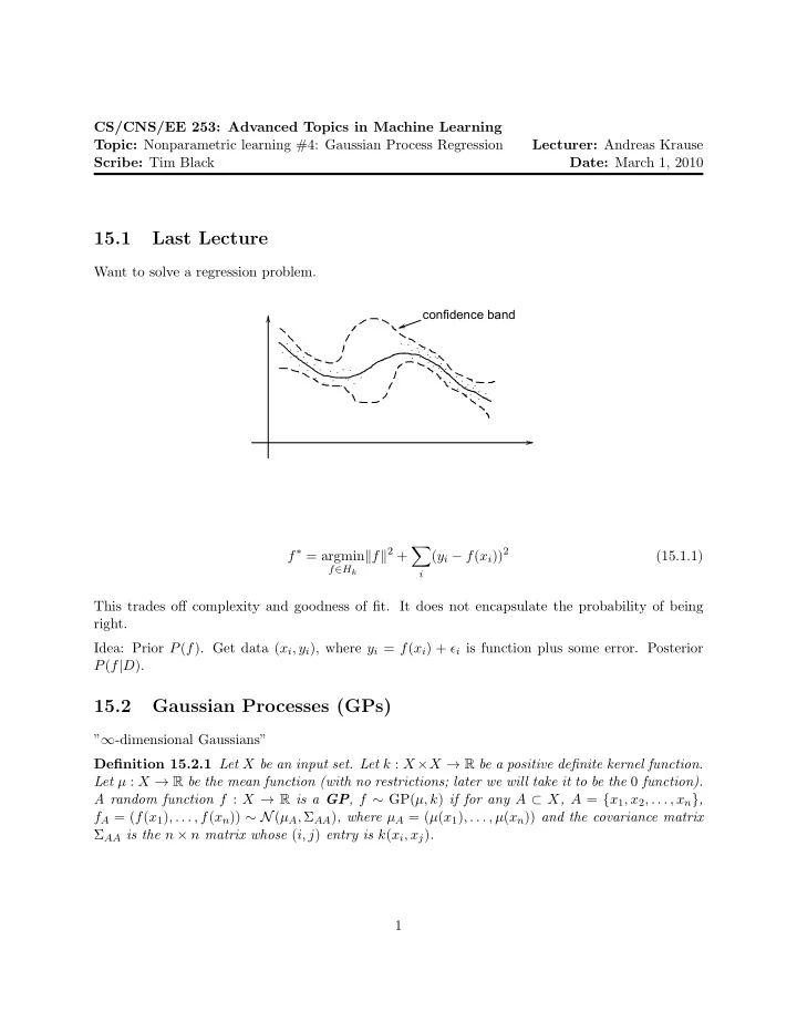
Want to solve a regression problem.

confidence band

f∗ = argmin

f∈Hk

f2 +

• i

(yi − f(xi))2 (15.1.1) This trades off complexity and goodness of fit. It does not encapsulate the probability of being right. Idea: Prior P(f). Get data (xi, yi), where yi = f(xi) + ǫi is function plus some error. Posterior P(f|D).

15.2 Gaussian Processes (GPs)

”∞-dimensional Gaussians” Definition 15.2.1 Let X be an input set. Let k : X ×X → R be a positive definite kernel function. Let µ : X → R be the mean function (with no restrictions; later we will take it to be the 0 function). A random function f : X → R is a GP, f ∼ GP(µ, k) if for any A ⊂ X, A = {x1, x2, . . . , xn}, fA = (f(x1), . . . , f(xn)) ∼ N(µA, ΣAA), where µA = (µ(x1), . . . , µ(xn)) and the covariance matrix ΣAA is the n × n matrix whose (i, j) entry is k(xi, xj). 1

f(x) x mean function covariance x f(x) (for set x) probability

• f f(x)

15.2.1 Prediction in GPs

Suppose we get to see fA = f′ (that is, we get to see the value of f at a set of points without noise). What is P(f(x)|fA = f′)? Conditionals on a Gaussian give a Gaussian: P(f(x)|fA = f′) = N(f(x); µx|A, σ2

x|A), where µx|A = µx + ΣxAΣ−1 AA(f′ − µA), σ2 x|A = σ2 x − ΣxAΣ−1 AAΣAx, and

ΣxA = (k(x, x1), k(x, x2), . . . , k(x, xn)). What if we have noise? yi = f(xi) + ǫi, ǫi ∼ N(0, Θ2) yA = fA + ǫA, ǫA ∼ N(0, σ2I) P(yA) = N(yA; µA, ΣAA + σ2

x|A)

P(f(x)|yA) = N(f(x); µx|A, σ2

x|A)

µx|A = µx + ΣxA(ΣAA + σ2I)−1(yA − µA) σ2

x|A = σ2 x + ΣxA(ΣAA + σ2I)−1ΣAx

NEVER EVER CALCULATE (ΣAA + σ2I)−1) AS inv(ΣAA + σ2I). Instead, solve the linear 2

system α = ˜ ΣAA(yA − µA) (Matlab notation), where ˜ ΣAA = ΣAA + σ2I, and α = ˜ Σ−1

AA(yA − µA).

15.2.2 Connection to RKHS

Assume µ = 0. µx|A = µx + ΣxA(ΣAA + σ2I)−1yA = n

i=1 αik(xi, x).

argmax

f∈Hk

P(f|yA) = argmin

f∈Hk

f2 + 1

σ2

• i(yi − f(xi))2.

15.2.3 Parameter Estimation

Most kernel functions have parameters. kSE(x, x′) = c2exp(− (x−x′)2

h

). Parameters are Θ = (c, h). c is the “magnitude” of the functions, and h is the “length scale” of f.

small h x x' k(x, x')

Let Nu = Number of upcrossings at level in [0, 1] (“How wiggly is this function”). Assume k is isotropic, k(x, x′) = k(x − x′), and assume µ = 0. 3

Theorem 15.2.2 (Adler). E[Nu] = 1 2π

• k′′(0)

k(0) exp

• − u2

2k(0)

• (15.2.2)

For SE kernel: k(0) = c2, k′′(0) = −2 c2

h2

E[Nu] =

1 2π

• 2

h2 exp

• − u2

2c2

• =

1 π √ 2 1 hexp

• − u2

2c2

• .

How do we choose the parameters? Learn from data! Pick parameters to maximize likelihood. Θ∗ = argmax

Θ

P(yA|Θ) = argmax

Θ

• P(yA, f|Θ)d

f = argmax

Θ

• P(yA|f, Θ)P(f|Θ)dΘ = argmax

Θ

• P(yA|f)P(f|Θ)dΘ

P(y |f) A P(f|O) high low low high high high

P(yA|Θ) = N(0, ΣAA(Θ) + σ2I) = (2π(ΣAA(Θ)))−n/2exp(− 1

2yT A(ΣAA(Θ) + σ2I)−1yA).

Solve the optimization problem by gradient descent. Θ∗ = argmax

Θ

P(yA|Θ) How do we solve it? Calculate gradient of log(P(yA|Θ)). Run conjugate gradient descent.

15.2.4 Incorporating prior knowlege

f = g + h ∼ GP(0, klin + kSE), where g is parametric and h is nonparametric. g(x) =

i wiφi(x). h ∼ GP(0, kSE). w ∼ N(0, I). g ∼ GP(0, klin). klin(x, x′) = i φi(x)φi(x′) =

φ(x)T φ(x′). 4