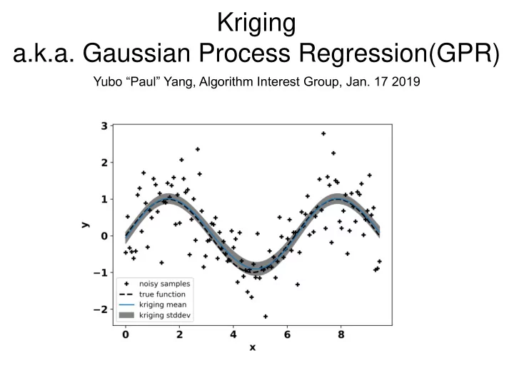
Kriging a.k.a. Gaussian Process Regression(GPR) Yubo Paul Yang, - - PowerPoint PPT Presentation

Kriging a.k.a. Gaussian Process Regression(GPR)

Yubo “Paul” Yang, Algorithm Interest Group, Jan. 17 2019

What is kriging?

Kriging is an interpolation method. Kriging minimizes the variance of prediction error at data points. Kriging provides uncertainty estimates to its predictions. ො 𝑧0 = 𝒙𝑈𝒛 𝐹[ො 𝑧0] = 𝐹[𝑧0] Minimize 𝑊[ො 𝑧0 − 𝑧0] Problem: Given samples of a random scalar field, predict value at un-sampled location. Solution: Design unbiased estimator with minimum prediction error variance.

Why krige?

Interpolation is generally useful. Error estimates on predictions. Gold! Photo by Sharon McCutcheon on Unsplash

How to krige? : ordinary

Derive ordinary kriging equation: assume stationary mean 𝐹 𝑧𝑗 = 𝜈, ∀𝑗 ො 𝑧0 = 𝒙𝑈𝒛 = ෍

𝑗=1 𝑂

𝑥𝑗 𝑧𝑗

[1] Wikipedia [2] Kriging Example [3] Ordinary Kriging by MSU Ashton Shortridge

• 1. Design unbiased estimator 𝐹[ො

𝑧0] = 𝐹 𝑧0 = 𝜈 𝐹 ො 𝑧0 = 𝐹 ෍

𝑗=1 𝑂

𝑥𝑗 𝑧𝑗 = ෍

𝑗=1 𝑂

𝑥𝑗 𝐹 𝑧𝑗 = 𝜈 ෍

𝑗=1 𝑂

𝑥𝑗 ෍

𝑗=1 𝑂

𝑥𝑗 = 1

• 2. Minimize prediction error variance 𝑊[ො

𝑧0 − 𝑧0] 𝑊 𝑧0 − ො 𝑧0 = 𝐷𝑝𝑤 𝑧0, 𝑧0 − 2𝐷𝑝𝑤 𝑧0, ො 𝑧0 + 𝐷𝑝𝑤[ො 𝑧0, ො 𝑧0] 𝐷𝑝𝑤 𝑧0, ො 𝑧0 = 𝐷𝑝𝑤 𝑧0, σ𝑗=1

𝑂

𝑥𝑗 𝑧𝑗 = σ𝑗=1

𝑂

𝑥𝑗𝐷𝑝𝑤[𝑧0, 𝑧𝑗] = 𝒙𝑈𝒆 𝑒𝑗 ≡ 𝐷𝑝𝑤[𝑧0, 𝑧𝑗] 𝐷𝑝𝑤 ො 𝑧0, ො 𝑧0 = 𝒙𝑈𝑫 𝒙 𝐷𝑗𝑘 ≡ 𝐷𝑝𝑤[𝑧𝑗, 𝑧𝑘] 𝑊 𝑧0 − ො 𝑧0 = 𝐷00 − 2𝒙𝑈𝒆 + 𝒙𝑈𝑫 𝒙

How to krige? : ordinary

Ordinary kriging equation: assume stationary mean 𝐹 𝑧𝑗 = 𝜈, ∀𝑗

[1] Wikipedia [2] Kriging Example [3] Ordinary Kriging by MSU Ashton Shortridge

σ𝑗=1

𝑂

𝑥𝑗 = 1 𝑊 𝑧0 − ො 𝑧0 = 𝐷00 − 2𝒙𝑈𝒆 + 𝒙𝑈𝑫 𝒙 minimize With the constaint 𝑫 𝟐 𝟐𝑈 𝒙 𝜇 = 𝒆 1 Solve ordinary kriging equation using Lagrange multiplier 𝜇 minimize 𝑊 𝑧0 − ො 𝑧0 − 2𝜇(𝟐𝑈𝒙 − 1)

How to krige? : ordinary

Ordinary kriging equation: assume stationary mean 𝐹 𝑧𝑗 = 𝜈, ∀𝑗

[1] Wikipedia [2] Kriging Example [3] Ordinary Kriging by MSU Ashton Shortridge

solution 𝜇 = 𝟐𝑈𝑫−1𝒆 − 1 𝟐𝑈𝑫−1𝟐 𝒙 = 𝑫−1(𝒆 − 𝜇𝟐) 𝑫 𝟐 𝟐𝑈 𝒙 𝜇 = 𝒆 1 result implementation 𝑊 ො 𝑧0 − 𝑧0 = 𝐷00 − 𝒙𝑈𝒆 − 𝜇 𝐹 ො 𝑧0 = 𝒙𝑈𝒛

How to krige? : simple

Simple kriging: assume 𝐹 𝑧𝑗 = 0, ∀𝑗 ⇒ no constraint on weights becomes 𝑫𝒙 = 𝒆 𝑫 𝟐 𝟐𝑈 𝒙 𝜇 = 𝒆 1 result implementation 𝑊 ො 𝑧0 − 𝑧0 = 𝐷00 − 𝒙𝑈𝒆 𝐹 ො 𝑧0 = 𝒙𝑈𝒛

The secret sauce: correlation function

The correlation function 𝐷𝑝𝑤(𝒚1, 𝒚2) should capture covariance in data. (CM people think g(r)) 𝐷𝑝𝑤(𝒚1, 𝒚2) is used to build the 𝑫 matrix and the 𝒆 vector. 𝐷𝑝𝑤(𝒚1, 𝒚2) is related to the so-called variogram by 𝛿 𝒚1, 𝒚2 = 𝐷𝑝𝑤 𝒚0, 𝒚0 − 𝐷𝑝𝑤(𝒚1, 𝒚2) Exponential sine squared 𝐷𝑝𝑤 𝒚1, 𝒚2 = exp −2 sin 𝜌 𝑈 𝒚1 − 𝒚2 𝑀

2

Squared exponential 𝐷𝑝𝑤 𝒚1, 𝒚2 = exp − 𝒚1 − 𝒚2 2 2𝑀2

The secret sauce: correlation function

Squared exponential 𝐷𝑝𝑤 𝒚1, 𝒚2 = exp − 𝒚1 − 𝒚2 2 2𝑀2

𝑀=1.5

Squared exponential 𝐷𝑝𝑤 𝒚1, 𝒚2 = exp − 𝒚1 − 𝒚2 2 2𝑀2

𝑀=5.0 A kriging expert knows how to choose the correlation function form and parameters.

Historical Review

Kriging was used for time series analysis back in the 1940s. Kriging got its name from Danie G. Krige’s master thesis for predicting the location of gold deposits in South Africa in 1960. Kriging is used extensively in geostatistics and meteorology. Kriging was reformulated in the context of Baysian inference in the late 1990s. Kriging is now known as Gaussian process regression. The choice of correlation function is phrased as a machine learning problem.

[1] Wikipedia [2] Chapter 2.8 RW2006

Gaussian Process

Gaussian process is the generalization of multivariate distribution to infinite variables. Gaussian process is probability distribution over functions.

Gaussian variable Normal distribution Gaussian vector Multivariate distribution Gaussian process

[1] Chapter 2.2 RW2006

Gaussian Process Regression

[1] Chris Fonnsbeck blog

Recent Applications

[1] A. P. Bartok et. al., “Machine Learning a General-Purpose Interatomic Potential for Silicon,” Phys. Rev. X 8, 041048 (2018). [2] A. Kamath et. al., “Neural networks vs Gaussian process regression for representing potential energy surfaces: A comparative study of fit quality and vibrational spectrum accuracy,” J. Chem. Phys. 148, 241702 (2018). [3] A. Denzel and J. Kastner, “Gaussian Process Regression for Transition State Search,” J. Chem. Theory Comput., 14 (11), pp 5777-5786 (2018). [4] G. Schmitz and O. Christiansen, “Gaussian process regression to accelerate geometry optimization relying on numerical differentiation,” J.

• Chem. Phys. 148, 241704 (2018).

Conclusions

Kriging is a minimal-variance unbiased interpolation algorithm. ො 𝑧0 = 𝒙𝑈𝒛 𝐹[ො 𝑧0] = 𝐹[𝑧0] Minimize 𝑊[ො 𝑧0 − 𝑧0] Problem: Given samples of a random scalar field, predict value at un-sampled location. Solution: Design unbiased estimator with minimum prediction error variance. Kriging result depends critically on the choice of correlation function (variogram). Kriging outputs a Gaussian process. Recently combined with Baysian inference and machine learning.