Overview Prediction with Gaussian Processes: Basic Ideas Bayesian - PowerPoint PPT Presentation

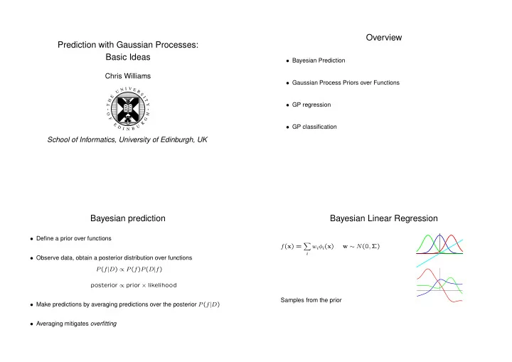
Overview Prediction with Gaussian Processes: Basic Ideas • Bayesian Prediction Chris Williams • Gaussian Process Priors over Functions I V N E U R S E I H T • GP regression Y T O H F G R E U • GP classification D I B N School of Informatics, University of Edinburgh, UK Bayesian prediction Bayesian Linear Regression • Define a prior over functions � f ( x ) = w i φ i ( x ) w ∼ N (0 , Σ) i • Observe data, obtain a posterior distribution over functions P ( f | D ) ∝ P ( f ) P ( D | f ) posterior ∝ prior × likelihood Samples from the prior • Make predictions by averaging predictions over the posterior P ( f | D ) • Averaging mitigates overfitting

Gaussian Processes: Priors over functions Examples of GPs • For a stochastic process f ( x ) , mean function is • σ 2 0 + σ 2 1 xx ′ µ ( x ) = E [ f ( x )] . Assume µ ( x ) ≡ 0 ∀ x • Covariance function k ( x , x ′ ) = E [ f ( x ) f ( x ′ )] . • exp −| x − x ′ | • Forget those weights! We should be thinking of defining priors over functions, not weights. • Priors over function-space can be defined directly by choosing a covariance function, e.g. • exp − ( x − x ′ ) 2 k ( x , x ′ ) = exp( − w | x − x ′ | ) • Gaussian processes are stochastic processes defined by their mean and covariance functions. Connection to feature space Gaussian process regression A Gaussian process prior over functions can be thought of as a Gaussian prior on the coefficients w ∼ N (0 , Λ) where i =1 , Gaussian likelihood p ( y i | f i ) ∼ N (0 , σ 2 ) Dataset D = ( x i , y i ) n N F � n f ( x ) = w i φ i ( x ) = w . Φ( x ) ¯ � f ( x ) = α i k ( x , x i ) i =1 i =1   φ 1 ( x ) where φ 2 ( x )   Φ( x ) = . α = ( K + σ 2 I ) − 1 y .   .   φ N F ( x ) In many interesting cases, N F = ∞ var( x ) = k ( x , x ) − k T ( x )( K + σ 2 I ) − 1 k ( x ) Choose Φ( · ) as eigenfunctions of the kernel k ( x , x ′ ) wrt p ( x ) (Mercer) � in time O ( n 3 ) , with k ( x ) = ( k ( x , x 1 ) , . . . , k ( x , x n )) T k ( x , y ) p ( x ) φ i ( x ) d x = λ i φ i ( y )

2.5 2 1.5 1 0.5 Y(x) 0 • Approximation methods can reduce O ( n 3 ) to O ( nm 2 ) for m ≪ n −0.5 −1 −1.5 −2 −2.5 0 0.1 0.2 0.3 0.4 0.5 0.6 0.7 0.8 0.9 1 After 1 observation: x • GP regression is competitive with other kernel methods (e.g. SVMs) 2.5 2 1.5 1 0.5 • Can use non-Gaussian likelihoods (e.g. Student-t) Y(x) 0 −0.5 −1 −1.5 −2 −2.5 0 0.1 0.2 0.3 0.4 0.5 0.6 0.7 0.8 0.9 1 After 2 observations: x Adapting kernel parameters • For GPs, the marginal likelihood (aka Bayesian evidence) log P ( y | θ ) can be optimized wrt the kernel parameters θ = ( v 0 , w ) d k ( x i , x j ) = v 0 exp − 1 l − x j l ) 2 w l ( x i • For GP regression log P ( y | θ ) can be computed exactly � 2 l =1 log P ( y | θ ) == − 1 2 log | K + σ 2 I | − 1 2 y T ( K + σ 2 I ) − 1 y − n 2 log 2 π w 1 = 5 . 0 w 2 = 5 . 0 w 1 = 5 . 0 w 2 = 0 . 5

Regularization Previous work • Wiener-Kolmogorov prediction theory (1940’s) • ¯ f ( x ) is the (functional) minimum of • Splines (Kimeldorf and Wahba, 1971; Wahba 1990) n 1 ( y i − f ( x i )) 2 + 1 2 � f � 2 � J [ f ] = • ARMA models for time-series H 2 σ 2 i =1 • Kriging in geostatistics (for 2-d or 3-d spaces) (1st term = − log-likelihood, 2nd term = − log-prior) • Regularization networks (Poggio and Girosi, 1989, 1990) • However, the regularization framework does not yield predictive variance • Design and Analysis of Computer Experiments (Sacks et al, 1989) or marginal likelihood • Infinite neural networks (Neal, 1995) GP prediction for classification problems • Likelihood − log P ( y i | f i ) = log(1 + e − y i f i ) 1 3 π f • Integrals can’t be done analytically – Find maximum a posteriori value of P ( f | y ) (Williams and Barber, 1997) −3 0 – Expectation-Propagation (Minka, 2001; Opper and Winther, 2000) Squash through logistic (or erf) function – MCMC methods (Neal, 1997)

MAP Gaussian process classification SVMs To obtain the MAP approximation to the GPC solution, we find ˆ f that maximizes the convex 1-norm soft margin classifier has the form function n n log(1 + e − y i f i ) − 1 y i α ∗ i k ( x , x i ) + w ∗ � � 2 f T K − 1 f + c f ( x ) = Ψ( y ) = − 0 i =1 i =1 where y i ∈ {− 1 , 1 } and α ∗ optimizes the quadratic form The optimization is carried out using the Newton-Raphson iteration n n f new = K ( I + WK ) − 1 ( W f + ( t − π )) α i − 1 � � Q ( α ) = t i t j α i α j k ( x i , x j ) where W = diag( π 1 (1 − π 1 ) , .., π n (1 − π n )) and π i = σ ( ˆ 2 f i ) . Basic complexity is O ( n 3 ) i =1 i,j =1 For a test point x ∗ we compute ¯ subject to the constraints f ( x ∗ ) and the variance, and make the prediction as � n P (class 1 | x ∗ , D ) = σ ( f ∗ ) p ( f ∗ | y ) d f ∗ � y i α i = 0 i =1 C ≥ α i ≥ 0 , i = 1 , . . . , n This is a quadratic programming problem. Can be solved in many ways, e.g. with interior point methods, or special purpose algorithms such as SMO. log(1 + exp(−z)) max(1−z, 0) 2 Basic complexity is O ( n 3 ) . 1 • Define g σ ( z ) = log(1 + e − z ) 0 −2 0 1 4 • SVM classifier is similar to GP classifier, but with g σ replaced by g SV M ( z ) = [1 − z ] + (Wahba, 1999) • Note that the MAP solution using g σ solution is not sparse, but gives a probability output