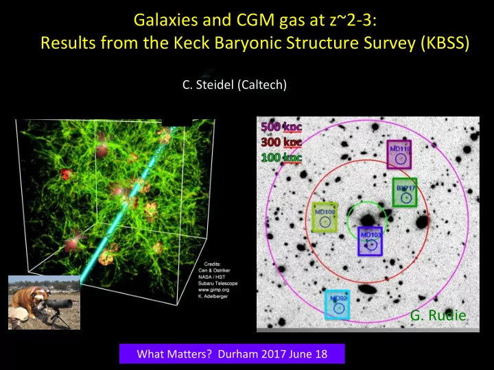
Galaxies and CGM gas at z~2-3: Results from the Keck Baryonic - PowerPoint PPT Presentation

Galaxies and CGM gas at z~2-3: Results from the Keck Baryonic Structure Survey (KBSS) C. Steidel (Caltech) G. Rudie What Matters? Durham 2017 June 18

“What Matters” Checklist 1. What is the origin and fate of the CGM? ✓ 2. What are the morphological and physical properties of the CGM? ✓ 3. What are the relevant physical processes on large (kpc) and small (pc) scales? ✓ 4. What is the relationship between CGM and galaxy properties? ✓ 5. How does the CGM evolve and what can we learn by comparing different epochs and tracers? ♪

Useful things to remember … When comparing CGM properties at low and high redshift: 1. Virial radius: • for DM halos with log(M h /M  )=12.0 – R vir ≈ 90 pkpc (z=2.5) – R vir ≈ 250 pkpc (z=0) 2.Correlation scales: • Beware co-moving vs. physical units (one and the same at z=0) – 1h -1 cMpc ≈ 1.4 cMpc = 1.40 pMpc (z=0) – 1h -1 cMpc ≈ 1.4 cMpc ≈ 0.35 pMpc (z=3)

Alternative Questions (with focus on high redshifts) A. How do galaxy-scale outflows affect/interact with accreting material (and when and where does it matter?) B. What is the expected metal content of wind material? Accreted material? C. How well-mixed are metals in CGM gas (vs. time)? D. What is the causal relationship (if any) between superwinds and CGM on 10- 500 kpc scales? How should we recognize the “smoking gun” when we see it? E. Outflows from galaxies are obviously multi-phase; to what extent are the low-ish ions most commonly observed good tracers of what is happening? F. What is the expected “fossil record” of past super-winds, as a function of time? G. Feedback from AGN vs. Stars/SNe :which, how, when, where? H. What is the impact of superwind-induced gas flows on stellar and gas-phase metallicity, on both short and long timescales?

Why z=2-3 is Optimal for Establishing Statistical Baselines for High Redshift Galaxies and their CGM • Peak of the “epoch of galaxy formation”, black hole accretion, blah, blah • The “magic” redshift range for diagnostic rest-optical nebular spectroscopy from terrestrial sites : z=2.1-2.6  n e , ionization, excitation, extinction, SFR, kinematics, chemistry; long heritage from nearby galaxy studies • Rest-frame far- UV can be observed without going to space, Lyα forest opacity is manageable • 3200-3730 Å : OVI @z=2.1-2.6 , higher Ly series • 3200-6000 Å Lya, Lyb, CII,CIII,CIV,SiII,SiIII,SiIV,NII,NV,etc. • L uv *  g’=24.0 at z=2.3: lots of galaxies to make the “grid”

“Bright Ages”? SFR “End of the Beginning”? T Madau & Dickinson 2014, ARAA M* “Mad Owl” Plot

Keck Baryonic Structure Survey ( [insert logo here] ) (2007-2017) • 15 independent fields, total solid angle of 0.25 deg 2, • Not GOODS, COSMOS, EGS, HUDF, CANDELS, etc. – each field centered on one of brightest QSOs in the entire sky with 2.55 < z < 2.85 • High density sampling of structure focused on 1.8 < z < 3.5 and (especially) z=2-2.6 • Intensive spectroscopy from UV to near-IR – 0.31- 0.80 μ Keck/HIRES (QSO spectroscopy, S/N~100) • 19 central QSOs in 15 fields – 0.32- 0.70 μ Keck/LRIS (KBSS -UV) • ~2400 with R~800-1500, covering ~1000-2000 Å in rest-frame – 1.15- 2.40 μ Keck/MOSFIRE (KBSS -MOSFIRE) • ~1200 galaxies, ~400 with J,H,K – 0.34-0.70 μ NB- selected Lyα Emitters (KBSS - Lyα) – - 10 of 15 fields, ~600 spectra (R=1500) – 0.35- 0.70 μ (LRIS -B+R)+ 1.1-2.4 μ (J,H,K) MOSFIRE (KBSS-LM) • R~1500 (rest UV), R~3600 (rest optical)

KBSS- 15 fields, 0.25 sq. degrees, ~4000 spectra <z>=2.4 ~2700 rest-UV spectra ~1300 rest-optical (MOSFIRE) spectra

Typical Field, 5.5’ x 7’, 184 spectroscopic redshifts , z~1.5-3.5 MOSFIRE KBSS 0100+13 z Q =2.721

Why did KBSS take ~10 years to get this to this point? 2 main reasons: 22

Reason 1. It is a lot of data; and, we had to take essentially all of it ourselves

Reason 2: MOSFIRE project timeline: Oct 2004 (start) - Sep 2012 (commissioning) MOSFIRE in the Caltech “Synchrotron” lab, just prior 12 to shipping (Feb. 2012) Photos: C. Johnson, UCLA

z=2.0-2.6 CS,Rudie,Strom+14

Resonance Lyman α photons scattered from “back” side of flow- acquire redshift with respect to stars Nebular emission lines Photons absorbed by from gas around gas moving toward forming stars- at rest with respect to galaxy observer, acquire redshift blueshift v astronomer

The View “Down the Barrel” (30 KBSS galaxies @ z~2.4) • <SFR> ≈ 30 M  /yr • <M * > ≈ 10 10 M  ; M DM ≈ 10 12 M  • <V c > ≈ 150 km/s • M gas > M * (gas-dominated) • Gas- phase O/H ≈ 0.5 solar • Stellar Fe/H ≈ 0.1 solar • Outflows: • extends to v max ≈ -1000 km/s • <v out > = -190 km/s • <v lya > = +290 km/s

Outflow kinematics of individual galaxies Q2343-BX418 Q2343-BX587 z=2.3054 z=2.2427

Ly α and H α in Faint Galaxies (z=2.57, R~27 in continuum (~0.1L*) Stack of 32 Ly α– selected galaxies, Hα+Lyα Hα (MOSFIRE) Lyα (LRIS -B) V (km/s relative to systemic) Trainor, CS + 2015

Densely Sampling the Universe @z~1.8-3.5: “Hi - Fi” Version Foreground Background QSO z

N HI > 10 14.5 cm -2 absorbers • > 4 times more likely to hit a log(N)>14.5 absorber near a galaxy than in the general IGM

HI Gas Around z=2.3 KBSS galaxies Rudie+2012 Galaxy Galaxy

The Physical State of the CGM Gas • Line width traces kinetic energy in the gas 2 + 2 kT 2 = b turb b d m • Increasing line width (turbulence?) with decreasing impact parameter Rudie+ 2012a

O VI KBSS Galaxy-centric 2-D maps of HI, 1000 metals 1.6 OVI 1.5 LOS Hubble distance [pMpc] 1.4 H I LOS velocity [km/s] Median (log 10 OVI ) 1.3 1.0 1000 1.2 1.2 1.0 1.1 Lyα LOS Hubble distance [pMpc] 0.8 100 1.0 LOS velocity [km/s] 0.6 Median (log 10 HI ) 0.9 0.4 1.0 0.8 0.2 0.7 0.0 0.1 0.6 100 0.2 0.1 1.0 0.4 Transverse distance [pMpc] C I V 0.6 2.9 0.8 1000 2.8 1.0 0.1 LOS Hubble distance [pMpc] 2.7 CIV 0.1 1.0 2.6 LOS velocity [km/s] Median (log 10 CIV ) Transverse distance [pMpc] 2.5 1.0 2.4 Turner+2014, KBSS-MOSFIRE 2.3 2.2 100 sample 2.1 2.0 Galaxy redshifts to σ≈ 15 km/s 1.9 1.8 0.1 0.1 1.0 Transverse distance [pMpc]

KBSS Galaxies and Dark Matter Halos in the EAGLE Simulations logM h >10.5 logM h >11.5 logM h >12.5 KBSS Ly α Typical halo masses of KBSS galaxies C IV independently estimated to be M h ~ 10 12 Si IV Turner+17 KBSS and EAGLE

Subtleties of OVI in the CGM of KBSS Galaxies Turner, Schaye, CS, Rudie, Strom 2015

The Smoking Gun of Galaxy Feedback?: • hot (>300,000 K) Gas within 200 kpc of forming galaxies… • near-solar metal content, and still moving at high velocity • <z>=2.4, <d>=140 kpc (physical). Turner, Schaye, CS, Rudie, Strom 2015

Corollaries • This hot phase is hard to identify, and easily masked by “normal” photoionized CGM material • Beware making assumptions about the mapping between HI and “over - density” - hot

Last Slide • The connection between the physical properties of forming galaxies during the peak of the galaxy formation era with the circumgalactic gas is eminently accessible to observation. • The “smoking gun” identified?– evidence for the direct influence of feedback , originating in the central, intensely star-forming regions -- on the larger-scale (200 kpc) properties of the CGM • “Recently disturbed” CGM is kinematically and chemically distinct from the more easily- observed, cooler CGM gas • Poor mixing between newly-formed metals and the larger CGM is indicated

KBSS-LM1: same 30 galaxies @z~2.4:

The Smoking Gun of Galaxy Feedback?: • hot (>300,000 K) Gas within 200 kpc of forming galaxies… • near-solar metal content, and still moving at high velocity • <z>=2.4, <d>=120 kpc (physical). Turner, Schaye, CS, Rudie, Strom 2015

z=2.3555 D gal =75 kpc, path separation ~ 0.4 kpc z=1.6265 DLA/LLS: Path Sep= ~1kpc

Q0100-BX210 • SFR~ 40 M  /yr • Log(M*/M  ) ~ 10.2 • O/H ~ 0.6 solar • 89 physical kpc from background QSO sightline HST-F140W

Low-Metallicity near the Systemic Velocity Rudie + in prep

Even Lower Metallicity at the Systemic Velocity Note the non-detection of CIV and SiIV

Near Solar Metallicity at Δ v~+200 km/s Rudie + in prep

Solar Metallicity at Δ v~-550 to -300 km/s Rudie + in prep

Orange: BPASSv2-300bin, Z=0.001, t=10 8 Cyan: same, reddened using Reddy,CS,+2016 extinction (Eldridge & Stanway 2016) CS+2017

z=3.05 Reddy, E(B-V)=0.137 A 1500 =1.22 (x 3.1) Z=3.05 SMC, E(B-V)=0.057 A 1500 =0.74 (x 2.0)

Z=2.4 Calzetti, E(B-V)=0.225 A 1500 =2.32 (x 8.5) Z=2.4 SMC, E(B-V)=0.09 A 1500 =1.17 (x 2.9)

MD27 2.8189 BX212 2.3782 2.4034 BX196 2.4918 BX196 2.4918 C12 2.9237 M11 3.1328 32.4114" C10 3.3913 BX195 2.3807 BX188 2.0602 BX18 BX186 2.357 016 0.0058 0.027 0.049 0.07 0.092 0.11 0.13 0.16 0.18 0.

Which absorbers trace the CGM? Rudie, CS, Trainor+12

KBSS-MOSFIRE: Nebular Excitation CS, Strom+2016; Strom, CS+2017