Formal approaches Static Graph v.s. Dynamic Behaviour to model - - PDF document

SLIDE 1

Formal approaches to model gene regulatory networks

Gilles Bernot

University of Nice sophia antipolis, I3S laboratory, France Acknowledgments: Observability Group of the Epigenomics Project

1

Menu

• 1. Modelling biological regulatory networks
• 2. Discrete framework for biological regulatory networks
• 3. Temporal logic and Model Checking for biology
• 4. Computer aided elaboration of formal models
• 5. Pedagogical example: Pseudomonas aeruginosa
• 6. Some current research topics
• 7. An extension to delays

2

Mathematical Models and Simulation

• 1. Rigorously encode sensible knowledge into ODEs for instance

2.

• A few parameters are approximatively known
• Some parameters are limited to some intervals
• Many parameters are a priori unknown
• 3. Perform lot of simulations, compare results with known

behaviours, and propose some credible values of the unknown parameters which produce acceptable behaviours

• 4. Perform additional simulations reflecting novel situations
• 5. If they predict interesting behaviours, propose new biological

experiments

• 6. Simplify the model and try to go further

3

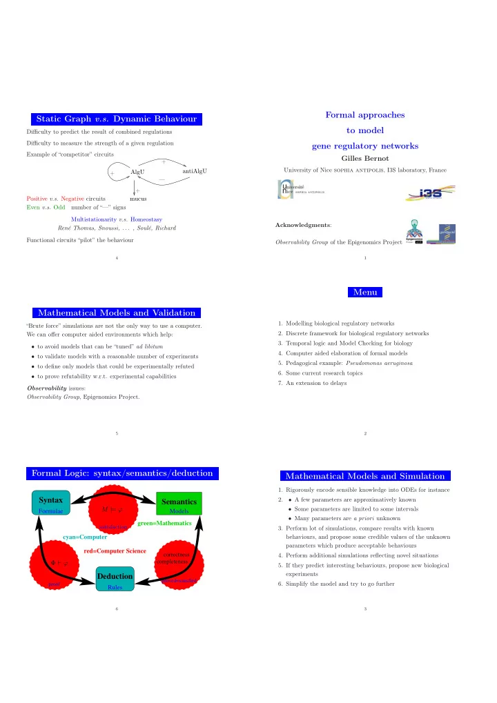
Static Graph v.s. Dynamic Behaviour

Difficulty to predict the result of combined regulations Difficulty to measure the strength of a given regulation Example of “competitor” circuits Positive v.s. Negative circuits

—

+ + AlgU antiAlgU mucus + Even v.s. Odd number of “—” signs Multistationarity v.s. Homeostasy René Thomas, Snoussi, . . . , Soulé, Richard Functional circuits “pilot” the behaviour

4

Mathematical Models and Validation

“Brute force” simulations are not the only way to use a computer. We can offer computer aided environments which help:

• to avoid models that can be “tuned” ad libitum
• to validate models with a reasonable number of experiments
• to define only models that could be experimentally refuted
• to prove refutability w.r.t. experimental capabilities

Observability issues: Observability Group, Epigenomics Project.

5

Formal Logic: syntax/semantics/deduction

cyan=Computer green=Mathematics

correctness

Rules

proof

Semantics

Models

Syntax Deduction

proved=satisfied

completeness

Formulae red=Computer Science M | = ϕ Φ ⊢ ϕ

satisfaction

6

SLIDE 2

Menu

• 1. Modelling biological regulatory networks
• 2. Discrete framework for biological regulatory networks
• 3. Temporal logic and Model Checking for biology
• 4. Computer aided elaboration of formal models
• 5. Pedagogical example: Pseudomonas aeruginosa
• 6. Some current research topics
• 7. An extension to delays

7

Multivalued Regulatory Graphs

y x x y 1 2 + + — —

x y x x

τ2 1 2 τ1

8

Regulatory Networks (R. Thomas)

Ky 1 2 —

x y

+ + 1 Basal level : Kx x helps : Kx,x Ky,x Absent y helps : Kx,y Both : Kx,xy (x,y) Focal Point (0,0) (Kx,y, Ky) (0,1) (Kx, Ky) (1,0) (Kx,xy, Ky) (1,1) (Kx,x, Ky) (2,0) (Kx,xy, Ky,x) (2,1) (Kx,x, Ky,x)

9

State Graphs

(x,y) Focal Point (0,0) (Kx,y, Ky)=(2,1) (0,1) (Kx, Ky)=(0,1) (1,0) (Kx,xy, Ky)=(2,1) (1,1) (Kx,x, Ky)=(2,1) (2,0) (Kx,xy, Ky,x)=(2,1) (2,1) (Kx,x, Ky,x)=(2,1)

y x

1

(1,1) (0,1) (0,0) (1,0) (2,0) (2,1)

1 2

“desynchronization” − →

by units of Manhattan distance

y x

1

(1,1) (1,0) (2,0) (2,1) (0,0) (0,1)

1 2 10

Menu

• 1. Modelling biological regulatory networks
• 2. Discrete framework for biological regulatory networks
• 3. Temporal logic and Model Checking for biology
• 4. Computer Aided elaboration Of Formal models
• 5. Pedagogical example: Pseudomonas aeruginosa
• 6. Some current research topics
• 7. An extension to delays

11

Time has a tree structure

y x

1

(1,1) (1,0) (2,0) (2,1) (0,0) (0,1)

1 2

As many possible state graphs as possible parameter sets. . . (huge number) From an initial state:

(2,1) (2,1) (1,1) (2,0) (1,0) (0,1) (0,0)

12

SLIDE 3

CTL = Computation Tree Logic

Atoms = comparaisons : (x=2) (y>0) . . . Logical connectives: (ϕ1 ∧ ϕ2) (ϕ1 = ⇒ ϕ2) · · · Temporal modalities: made of 2 characters first character second character A = for All path choices X = neXt state F = for some Future state E = there Exist a choice G = for all future states (Globally) U = Until

AX(y = 1) : the concentration level of y belongs to the interval 1 in all states directly following the considered initial state. EG(x = 0) : there exists at least one path from the considered initial state where x always belongs to its lower interval.

13

Temporal Connectives of CTL

neXt state: EXϕ : ϕ can be satisfied in a next state AXϕ : ϕ is always satisfied in the next states eventually in the Future: EFϕ : ϕ can be satisfied in the future AFϕ : ϕ will be satisfied at some state in the future Globally: EGϕ : ϕ can be an invariant in the future AGϕ : ϕ is necessarilly an invariant in the future Until: E[ψUϕ] : there exist a path where ψ is satisfied until a state where ϕ is satisfied A[ψUϕ] : ψ is always satisfied until some state where ϕ is satisfied

14

Semantics of Temporal Connectives

t+1 ϕ

AXϕ

ϕ ϕ ϕ ϕ ϕ ϕ t+1 ϕ

EXϕ

t t t ϕ t t+k

EFϕ ... ... ... ... ... ... ... ... AGϕ ... EGϕ ... AFϕ

ϕ ϕ ϕ ϕ ϕ

E[ψUϕ] A[ψUϕ] ... ... ... ...

15

CTL to encode Biological Properties

Common properties: “functionality” of a sub-graph Special role of “feedback loops”

—

y

+ +

x

1 2 1

– positive: multistationnarity (even number of — ) – negative: homeostasy (odd number of — ) y x y x

(0,1) (2,1) (1,1) (2,0) (0,0) (1,0) (0,0) (1,0) (2,0) (2,1) (1,1) (0,1)

Characteristic properties:    (x = 2) = ⇒ AG(¬(x = 0)) (x = 0) = ⇒ AG(¬(x = 2)) They express “the positive feedback loop is functional” (satisfaction of these formulae relies on the parameters K...)

16

Model Checking

Efficiently computes all the states of a state graph which satisfy a given formula: { η | M | =η ϕ }. Efficiently select the models which globally satisfy a given formula.

17

Model Checking for CTL

Computes all the states of a theoretical model which satisfy a given formula: { η | M | =η ϕ }. Idea 1: work on the state graph instead of the path trees. Idea 2: check first the atoms of ϕ and then check the connectives of ϕ with a bottom-up computation strategy. Idea 3: (computational optimization) group some cases together using BDDs (Binary Decision Diagrams). Example : (x = 0) = ⇒ AG(¬(x = 2)) Obsession: travel the state graph as less as possible

18

SLIDE 4

(x = 0) = ⇒ AG(¬(x = 2))

x=0 x=2 z ¬(x = 2) z x y x y

and AG(¬(x = 2)) ? . . . one should travel all the paths from any green box and check if successive boxes are green: too many boxes to visit. Trick: AG(¬(x = 2)) is equivalent to ¬EF(x = 2) start from the red boxes and follow the transitions backward.

19

Theoretical Models ↔ Experiments

CTL formulae are satisfied (or refuted) w.r.t. a set of paths from a given initial state

• They can be tested against the possible paths of the theoretical

models (M | =Model Checking ϕ)

• They can be tested against the biological experiments

(Biological_Object | =Experiment ϕ) CTL formulae link theoretical models and biological objects together

20

Menu

• 1. Modelling biological regulatory networks
• 2. Discrete framework for biological regulatory networks
• 3. Temporal logic and Model Checking for biology
• 4. Computer aided elaboration of formal models
• 5. Pedagogical example: Pseudomonas aeruginosa
• 6. Some current research topics
• 7. An extension to delays

21

Computer Aided Elaboration of Models

From biological knowledge and/or biological hypotheses, it comes:

• properties:

“Without stimulus, if gene x has its basal expression level, then it remains at this level.”

• model schemas:

—

y

+ +

x

1 2 1

—

x y

+ +

2 1 1

. . . Formal logic and formal models allow us to:

• verify hypotheses and check consistency
• elaborate more precise models incrementally
• suggest new biological experiments to efficiently reduce the

number of potential models

22

The Two Questions

Φ = {ϕ1, ϕ2, · · · , ϕn} and M =

—

y

+ +

x

1 2 1

. . .

• 1. Is it possible that Φ and M ?

Consistency of knowledge and hypotheses. Means to select models belonging to the schemas that satisfy Φ. (∃? M ∈ M | M | = ϕ)

• 2. If so, is it true in vivo that Φ and M ?

Compatibility of one of the selected models with the biological

• bject. Require to propose experiments to validate or refute

the selected model(s). → Computer aided proofs and validations

23

Question 1 = Consistency

• 1. Draw all the sensible regulatory graphs with all the sensible

threshold allocations. It defines M.

• 2. Express in CTL the known behavioural properties as well as

the considered biological hypotheses. It defines Φ.

• 3. Automatically generate all the possible regulatory networks

derived from M according to all possible parameters K.... Our software plateform SMBioNet handles this automatically.

• 4. Check each of these models against Φ.

SMBioNet uses model checking to perform this step.

• 5. If no model survive to the previous step, then reconsider the

hypotheses and perhaps extend model schemas. . .

• 6. If at least one model survives, then the biological hypotheses

are consistent. Possible parameters K... have been indirectly

• established. Now Question 2 has to be addressed.

24

SLIDE 5

Generation of biological experiments (1)

Set of all the formulae: ϕ = hypothesis

ϕ

25

Generation of biological experiments (2)

Set of all the formulae: ϕ = hypothesis Obs = possible experiments

Obs ϕ

26

Generation of biological experiments (3)

Set of all the formulae: ϕ = hypothesis Obs = possible experiments Th(ϕ) = ϕ inferences

Obs ϕ

27

Generation of biological experiments (4)

Set of all the formulae: ϕ = hypothesis Obs = possible experiments Th(ϕ) = ϕ inferences S = sensible experiments

Obs ϕ S

28

Generation of biological experiments (5)

Set of all the formulae: ϕ = hypothesis Obs = possible experiments Th(ϕ) = ϕ inferences S = sensible experiments Refutability: S = ⇒ ϕ ?

Obs ϕ S

29

Generation of biological experiments

Set of all the formulae: ϕ = hypothesis Obs = possible experiments Th(ϕ) = ϕ inferences S = sensible experiments Refutability: S = ⇒ ϕ ? Best refutations: Choice of experiments in S ? . . . optimisations

Obs ϕ S

30

SLIDE 6

Question 2 = Validation

• 1. Among all possible formulae, some are “observable” i.e., they

express a possible result of a possible biological experiment. Let Obs be the set of all observable formulae.

• 2. Let Λ be the set of theorems of Φ and M.

Λ ∩ Obs is the set of experiments able to validate the survivors

• f Question 1. Unfortunately it is infinite in general.
• 3. Testing frameworks from computer science aim at selecting a

finite subsets of these observable formulae, which maximize the chance to refute the survivors.

• 4. These subsets are often too big, nevertheless these testing

frameworks can be suitably applied to regulatory networks. It has been the case of the mucus production of P.aeruginosa.

31

Menu

• 1. Modelling biological regulatory networks
• 2. Discrete framework for biological regulatory networks
• 3. Temporal logic and Model Checking for biology
• 4. Computer aided elaboration of formal models
• 5. Pedagogical example: Pseudomonas aeruginosa
• 6. Some current research topics
• 7. An extension to delays

32

Mutation, Epigenesis, Adaptation

Terminology about phenotype modification: genetic modification: inheritable and not reversible (mutation) epigenetic modification: inheritable and reversible adaptation: not inheritable and reversible The biological question (Janine Guespin): is mucus production in Pseudomonas aeruginosa due to an epigenetic switch ? = ⇒ New possible therapy [→ cystic fibrosis]

33

Mucus Production in P. aeruginosa

Capture:

• peron

self−inducer abstract behaviour — + AlgU antiAlgU mucus + + membrane AlgU AntiAlgU AntiAlgU AlgU AlgU

34

Parameters & thresholds: unknown

Thresholds for AlgU in P.aeruginosa are unknown:

—

+ +

—

+ +

—

+ + antiAlgU AlgU AlgU AlgU antiAlgU antiAlgU

1 1 1 1 1 1 1 2 2

and parameters are unknown: 34 × 22 34 × 22 24 × 22 712 possible models One CTL formula for each stable state: (AlgU = 2) = ⇒ AXAF(AlgU = 2) (AlgU = 0) = ⇒ AG(¬(AlgU = 2)) Question 1, consistency: proved by Model Checking → 10 models among the 712 models are extracted by SMBioNet

35

Validation of the epigenetic hypothesis

Question 2 = to validate bistationnarity in vivo Non mucoid state: (AlgU = 0) = ⇒ AG(¬(AlgU = 2))

• P. aeruginosa, with a basal level for AlgU does not produce mucus

spontaneously: actually validated Mucoid state: (AlgU = 2) = ⇒ AXAF(AlgU = 2) Experimental limitation: AlgU can be saturated but it cannot be measured. Experiment: to pulse AlgU and then to test if mucus production remains (⇐ ⇒ to verify a hysteresis) This experiment can be generated automatically

36

SLIDE 7

To test (AlgU=2)= ⇒AXAF(AlgU=2)

AlgU = 2 cannot be directly verified but mucus = 1 can be verified.

—

+ + AlgU antiAlgU mucus + Lemma: AXAF(AlgU = 2) ⇐ ⇒ AXAF(mucus = 1) (. . . formal proof by computer . . . ) → To test: (AlgU = 2) = ⇒ AXAF(mucus = 1)

37

(AlgU = 2) = ⇒ AXAF(mucus = 1)

A = ⇒ B true false true true false false true true

Karl Popper: to validate = to try to refute thus A=false is useless experiments must begin with a pulse The pulse forces the bacteria to reach the initial state AlgU = 2. If the state were not directly controlable we had to prove lemmas: (something reachable) = ⇒ (AlgU = 2) General form of a test: (something reachable) = ⇒ (something observable)

38

Menu

• 1. Modelling biological regulatory networks
• 2. Discrete framework for biological regulatory networks
• 3. Temporal logic and Model Checking for biology
• 4. Computer aided elaboration of formal models
• 5. Pedagogical example: Pseudomonas aeruginosa
• 6. Some current research topics
• 7. An extension to delays

39

Research topics (1)

Explicit singular states:

y

1 1

x

( 1 , 0 ) ( 0 , 0 ) ( 0 , 1 ) ( 1 , 1 )

y x

|1,1| |1,1| |0,0| |0,0|

( |0,0| , |0,0| ) ( |0,0| , |0,1| )

|0,1| |0,1|

( |0,0| , |1,1| ) ( |1,1| , |0,0| ) ( |1,1| , |1,1| ) ( |0,1| , |0,1| )( |1,1| , |0,1| ) ( |0,1| , |0,0| ) ( |0,1| , |1,1| )

e.g. to distinguish stable states from limit cycles

40

Research topics (2)

Hybrid approaches: simplified trajectories which locally approximate differential equations

y

1 1

x

( 1 , 0 ) ( 0 , 0 ) ( 0 , 1 ) ( 1 , 1 )

y

1 1

x

(e.g. linear)

41

Research topics (4)

Stochastic approaches:

y

1 1

x

p1 p2

More or less dual to delays

42

SLIDE 8

Research topics (5)

Networks with multiplexes:

y x z x z y

(y ∧ z) ∧ ¬x

– + +

Explicit encoding of knowledge on cooperations

43

Research topics (6)

From static shapes to properties on dynamics:

• positive/negative cycles and epigenesis/homeostasis
• maximum number of attraction basins
• . . .

Mathematical proofs similar to the ones for cellular automaton

44

Research topics (7)

Embeddings of Regulatory Networks:

x y z t u v x y z t u v Preserved behaviour ? Studied behaviour

Necessary and sufficient condition on the local dynamics of the “input frontier” Offers a methodology to identify interesting sub-networks

45

Research topics (3)

Time delays:

y

1 1

x

( 1 , 0 ) ( 0 , 0 ) ( 0 , 1 ) ( 1 , 1 )

x y

1 1

(size of rectangular areas = delays) Requires constraint solving

46

Menu

• 1. Modelling biological regulatory networks
• 2. Discrete framework for biological regulatory networks
• 3. Temporal logic and Model Checking for biology
• 4. Computer aided elaboration of formal models
• 5. Pedagogical example: Pseudomonas aeruginosa
• 6. Some current research topics
• 7. An extension to delays

47

Ambiguous discrete models

y x y x y x y x

?

1 1 2

1 ou 2 attraction basins ? It depends on the relative delays for x and y to cross each of the four domains.

48

SLIDE 9

Regulatory Network with Delays

N = (V, E, K, D) – As usual : bounded variables (V ), edges with sign and threshold (E), family of parameters (K) – Production and degradation delays : D = D+ ∪ D− — D+ = {δ+

v,iω}v∈V,i∈[0,Kv,ω],ω⊂G−1(v)

— D− = {δ−

v,iω}v∈V,i∈[Kv,ω,bv],ω⊂G−1(v)

Delays vary in I R+ according to the current state (i) and the resources (ω) of a variable v

49

Dynamics within a unique domain

A state : η = (l, d) where l : V → I N is a discrete state as usual and d : V → I R+ satisfies : d(v) ≤ δ+

v,l(v)ωl(v) + δ− v,l(v)ωl(v) d d d when k > i the moving delay is δ+

v,ik − d in the

δ+

v,ik

direction of v (horizontal) when k < i the moving delay is d in the δ−

v,ik

direction of v (horizontal) d d when k = i the moving delay is |δ+

v,ik − d| in the

direction of v (horizontal) δ+

v,i

δ−

v,i

d

Moving delay : µη(v) = |δ+

v,l(v)ωl(v) − d(v)| 50

Dynamics

η′ = (l′, d′) is a successor of η = (l, d) iff ∃u ∈ V s.t.: – ∀v ∈ V, µη(u) ≤ µη(v) – l′(u) = l(u) + κη(u) with κη(u) ∈ {−1, 0, 1} as usual – ∀v ∈ V, u = v = ⇒ l′(v) = l(v) – κη(u) = 0 = ⇒ (∀v ∈ V, d′(v) = δ+

v,l(v)ωl(v))

– κη(u) = 0 = ⇒ d′(u) = 0 – κη(u) = 0 = ⇒ ( ∀v ∈ V, u = v = ⇒ d′(v) =

(d(v)+µη(u) × (δ+

v,l′(v)ωl′ (v)+δ− v,l′(v)ωl′ (v))

δ+

v,l(v)ωl(v)+δ− v,l(v)ωl(v)

)

51

Dynamics = Thales in the space of delays

if all cross delays are infinite then the regular state is stable δ+

v,i

δ−

v,i

δ+

u,j

δ−

u,j

state η where u is the modified variable d(v) + µη(u) d′(v) successor state η′ with l′(u) = l(u) + κη(u)

δ+

v,l′(v)ωl′(v) + δ− v,l′(v)ωl′(v)

δ+

v,l(v)ωl(v) + δ− v,l(v)ωl(v) 52

Concluding Comments

Models to encode already elucidated biological models v.s. modelling methods to help discovery in biology. . . Behavioural properties (Φ) are as much important as models (M) Modelling is significant only with respect to the considered experimental reachability and observability (Obs) Formal proofs can suggest wet experiments

• But. . .

even very simple approaches for delays are unreachable for model checking : we currently explore constraint programming methods.

53