Fixed Points meet Lbs Rule Fefermans G2 plus Examples Uniform - - PowerPoint PPT Presentation

Feferman’s G2 plus Examples Uniform Semi-numerability The Henkin Calculus The µ-Calculus

1

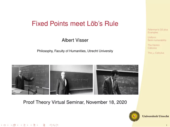
Fixed Points meet Löb’s Rule

Albert Visser

Philosophy, Faculty of Humanities, Utrecht University

Proof Theory Virtual Seminar, November 18, 2020

Feferman’s G2 plus Examples Uniform Semi-numerability The Henkin Calculus The µ-Calculus

2

Overview

Feferman’s G2 plus Examples Uniform Semi-numerability The Henkin Calculus The µ-Calculus

Feferman’s G2 plus Examples Uniform Semi-numerability The Henkin Calculus The µ-Calculus

2

Overview

Feferman’s G2 plus Examples Uniform Semi-numerability The Henkin Calculus The µ-Calculus

Feferman’s G2 plus Examples Uniform Semi-numerability The Henkin Calculus The µ-Calculus

2

Overview

Feferman’s G2 plus Examples Uniform Semi-numerability The Henkin Calculus The µ-Calculus

Feferman’s G2 plus Examples Uniform Semi-numerability The Henkin Calculus The µ-Calculus

2

Overview

Feferman’s G2 plus Examples Uniform Semi-numerability The Henkin Calculus The µ-Calculus

Feferman’s G2 plus Examples Uniform Semi-numerability The Henkin Calculus The µ-Calculus

3

Overview

Feferman’s G2 plus Examples Uniform Semi-numerability The Henkin Calculus The µ-Calculus

Feferman’s G2 plus Examples Uniform Semi-numerability The Henkin Calculus The µ-Calculus

4

Feferman’s G2

We fix an arithmetisation “proof(X, x, y)” for “x is a proof of y from axioms in X”. Here X is a unary predicate symbol. We write provα(y) for ∃x proof(α, x, y).

Theorem (± Feferman 1960)

Consider any consistent RE theory T and an interpretation K of EA + BΣ1 in T. Suppose σ is Σ1 and σK semi-numerates the axioms of T in T. Then, we have T (con(σ))K. One can omit BΣ1, but then we need a modification of the proof.

Feferman’s G2 plus Examples Uniform Semi-numerability The Henkin Calculus The µ-Calculus

5

Limitations

◮ We have G2 for oracle provability, the provability notion

associated with ω-consistency, cut-free EA-provability over EA, etcetera.

◮ EA + BΣ1 seems far too strong to be a convincing base

theory.

◮ The role of the very specific formula-class Σ1.

We provide a more general Feferman-style result that works for certain predicates of the form provα that do not satisfy the Löb conditions.

Feferman’s G2 plus Examples Uniform Semi-numerability The Henkin Calculus The µ-Calculus

6

The (non-)Role of the Löb Conditions

Feferman’s proof employs the Löb Conditions for provK. There is a Σ0

1-numeration σ of the axioms of EA in EA such that:

◮ EA ⊢ ∃x ∀y ∈ σ y < x. ◮ EA

σ σ ⊤ ↔ σ ⊥.

◮ EA ⊢ G ↔

σ σ ⊥, for any G with EA ⊢ G ↔ ¬ σ G.

So the Löb Conditions fail for EA. However, the result, G2 for Σ1-semi-numerations, does hold —as follows from result below.

Feferman’s G2 plus Examples Uniform Semi-numerability The Henkin Calculus The µ-Calculus

7

Numerability is not Sufficient

An Example due to Feferman. Let π be a standard predicate representing the axioms of PA. Let πx(y) :↔ π(y) ∧ y ≤ x. We define π⋆(y) :↔ π(y) ∧ con(πy). Note that π⋆ is Π0

1.

π⋆ numerates the axioms of PA in PA, but we do have PA ⊢ con(π⋆). To verify in PA that the first k axioms are indeed axioms we need axioms enumerated after stage k. Thus, the restriction to Σ1 is needed in Feferman’s Theorem.

Feferman’s G2 plus Examples Uniform Semi-numerability The Henkin Calculus The µ-Calculus

8

Overview

Feferman’s G2 plus Examples Uniform Semi-numerability The Henkin Calculus The µ-Calculus

Feferman’s G2 plus Examples Uniform Semi-numerability The Henkin Calculus The µ-Calculus

9

Uniform Semi-numerability

What goes wrong in Feferman’s Example is all that goes wrong. We fix proof(X, x, y). Consider a consistent theory U. Let X be the set of (Gödel numbers of) axioms of U. There are no constraints on the complexity of X. Let Uk be axiomatised by Xk, the elements of X that are ≤ k. Suppose N : S1

2 U.

A U-formula ξ uniformely semi-numerates X (w.r.t. N) iff, for every n, there is an m ≥ n, such that Um proves ξ(i), for each i ∈ Xm.

Feferman’s G2 plus Examples Uniform Semi-numerability The Henkin Calculus The µ-Calculus

10

A General Version of G2

Theorem

Suppose U is consistent and ξ uniformly semi-numerates the axioms X of U (w.r.t. N). Then, U conN[ξ]. The square brackets emphasise that ξ is not supposed to be relativised to N. Let B be a single sentence that axiomatises S1

2.

Proof.

Suppose U ⊢ conN[ξ]. Then, for some k, Uk ⊢ BN ∧ conN[ξ] and ξ semi-numerates Xk in Uk. Let β :=

A∈Xk (x = A). We find

Uk ⊢ (B ∧ con(β))N. This contradicts a standard version of G2. ❑ provN

[ξ] need not to satisfy the Löb Conditions. Yet the Löb

Condtions are used in the proof.

Feferman’s G2 plus Examples Uniform Semi-numerability The Henkin Calculus The µ-Calculus

11

Löb’s Rule

Since, uniformity can be easily lifted to finite extensions, we have:

Theorem

Suppose ξ uniformly semi-numerates the axioms of U (w.r.t. N) and U ⊢ provN

[ξ](A) → A. Then U ⊢ A.

Feferman’s G2 plus Examples Uniform Semi-numerability The Henkin Calculus The µ-Calculus

12

Overview

Feferman’s G2 plus Examples Uniform Semi-numerability The Henkin Calculus The µ-Calculus

Feferman’s G2 plus Examples Uniform Semi-numerability The Henkin Calculus The µ-Calculus

13

The Henkin Calculus

We work in the language of modal logic extended with a fixed-point

• perator ̥p.

ϕ. HC has the following axioms and rules.

◮ The axioms and rules of K, ◮ Löb’ rule: if ⊢

ϕ → ϕ, then ⊢ ϕ.

◮ If ψ results from ϕ by renaming bound variables, then

⊢ ϕ ↔ ψ.

◮ If ̥p.

ϕ is substitutable for p in ϕ, then ⊢ ̥p. ϕ ↔ ϕ[p : ̥p. ϕ].

Feferman’s G2 plus Examples Uniform Semi-numerability The Henkin Calculus The µ-Calculus

14

Perspective

The Henkin Calculus has standard syntax here. The disadvantage is that one has to get the details for variable-binding right —as is witnessed by the presence of the α-equivalence axiom. One gets a sense that this material is about circularity rather than

• binding. A treatment using syntax on possibly cyclic graphs seems

to represent what is going on much better. Such a treatment would be co-inductive. The disadvantage is discontinuity with conventional treatments. The disadvantage of the second approach can, hopefully, be

• vercome by metatheorems linking the conventional treatment to

the co-inductive one.

Feferman’s G2 plus Examples Uniform Semi-numerability The Henkin Calculus The µ-Calculus

15

Circular Henkin Calculus

This is what the Henkin Calculus looks like on directed possibly circular graphs. Note that ̥ is not in the language here. We demand that in a graph that represents a formula every cycle contains a vertex labeled with a box. This is the guarding condition.

◮ The Axioms and Rules of K. ◮ Löb’s rule: if ⊢

ϕ → ϕ, then ⊢ ϕ.

◮ If ϕ and ψ are bisimilar then ⊢ ϕ ↔ ψ.

Feferman’s G2 plus Examples Uniform Semi-numerability The Henkin Calculus The µ-Calculus

16

The Grullet Modality

Back to the ordinary syntax. We define:

◮

• ϕ := ̥p. (ϕ ∧ p), where p is not free in ϕ.

We have:

◮ HC ⊢

• ϕ ↔

(ϕ ∧

• ϕ).

◮ HC verifies Löb’s Logic for

• .

◮ Suppose ϕ is modalised in p, then

HC ⊢ (•(p ↔ ϕ) ∧ •(q ↔ ϕ[p : q])) → (p ↔ q). A version of the De Jongh-Sambin-Bernardi Theorem Gödel and Henkin sentences are unique.

Feferman’s G2 plus Examples Uniform Semi-numerability The Henkin Calculus The µ-Calculus

17

Multiple Fixed Points 1

Consider a system of equations E given by: (p0 ↔ ϕ0), . . . , (pn−1 ↔ ϕn−1), We assign a directed graph GE to E with as nodes the variables pi, for i < n. We have an arrow from pi to pj iff there is an unguarded free occurrence of pj in ϕi. E is guarded iff GE is acyclic. If E is guarded, it has a unique solution. In this solution the free variables are those of the ϕi minus the pj.

Feferman’s G2 plus Examples Uniform Semi-numerability The Henkin Calculus The µ-Calculus

18

Multiple Fixed Points 2

Figure: The associated graph

Feferman’s G2 plus Examples Uniform Semi-numerability The Henkin Calculus The µ-Calculus

19

Reduction

Suppose ϕ is modalised in p. We can find a ϕ and fresh q0, . . . , qn−1, such that p does not occur in ϕ and HC ⊢ ϕ ↔ ϕ [q0 : ψ0, . . . , qn−1 : ψn−1]. By solving the equations E : p ↔ ϕ, q0 ↔ ψ0, . . . , qn−1 ↔ ψn−1. we see that ϕ has a unique fixed point.

Feferman’s G2 plus Examples Uniform Semi-numerability The Henkin Calculus The µ-Calculus

20

The Extended Henkin Calculus

Using the reduction result we can show that the Henkin Calculus is synonymous with its extended variant where we have fixed points for modalised formulas:

◮ we have ̥p.ϕ in case p only occurs in the scope of a box.

The axioms for the extended calculus are analogous. On the circular syntax the difference between both versions disappears.

Feferman’s G2 plus Examples Uniform Semi-numerability The Henkin Calculus The µ-Calculus

21

Arithmetical Interpretation

Suppose ξ uniformly semi-numerates the axioms of U w.r.t N. Then, HC is arithmetically valid in U for provN

[ξ].

The precise interpretation of the fixed-point operator and the proof

• f soundness take some doing.

Feferman’s G2 plus Examples Uniform Semi-numerability The Henkin Calculus The µ-Calculus

22

Completeness

HC and extended HC both have a Kripke model completeness theorem in finite dags and in finite trees. Is the provability logic of all uniformely semi-numerable axiom sets precisely HC? If so, is there a pair U, α, where this logic is assumed? It is a win-win situation: how cool would it be to find an extra principle.

Feferman’s G2 plus Examples Uniform Semi-numerability The Henkin Calculus The µ-Calculus

23

Overview

Feferman’s G2 plus Examples Uniform Semi-numerability The Henkin Calculus The µ-Calculus

Feferman’s G2 plus Examples Uniform Semi-numerability The Henkin Calculus The µ-Calculus

24

The µ-Calculus

Our version of the µ-calculus consists of K plus fixed points for formulas in which the fixed-point-variable occurs positively. We write µp for the fixed-point operator reflecting our intention to look at minimal fixed points. We have the following axiom expressing minimality:

◮ ⊢ ϕ[p : α] → α

⇒ ⊢ µp.ϕ → α. The well-founded part of µ is µ + H, where H := µp. p. µ + H is synonymous with HC.

Feferman’s G2 plus Examples Uniform Semi-numerability The Henkin Calculus The µ-Calculus

25

Well-Foundedness beats Negativity 1

Consider ϕ modalised in p. Let ϕ0 be the result of replacing all negative occurrences of p in ϕ by a fresh q. Let ϕ1 be the result of replacing all positive occurrences of p in ϕ by q. A solution lemma tells us that the equations p ↔ ϕ0, q ↔ ϕ1 in µ can be solved. Let the solutions be α0 and α1.

Feferman’s G2 plus Examples Uniform Semi-numerability The Henkin Calculus The µ-Calculus

26

Well-Foundedness beats Negativity 2

In µ + H, we have uniqueness of modalised fixed points for systems of equations and, hence µ + H ⊢ α0 ↔ α1. Ergo µ + H ⊢ α0 ↔ ϕ0[p : α0, q : α0], so α0 is a fixed point of ϕ.

Feferman’s G2 plus Examples Uniform Semi-numerability The Henkin Calculus The µ-Calculus

27

Thank You