Finite-size scaling For a system of length L, the correlation length - - PowerPoint PPT Presentation

▶

Aug 17, 2022 280 likes •436 views

Finite-size scaling For a system of length L, the correlation length Express divergent quantities in terms of correlation length, e.g., The largest value is obtained by substituting At what T does the maximum occur? The peak position of a

SLIDE 1

Finite-size scaling

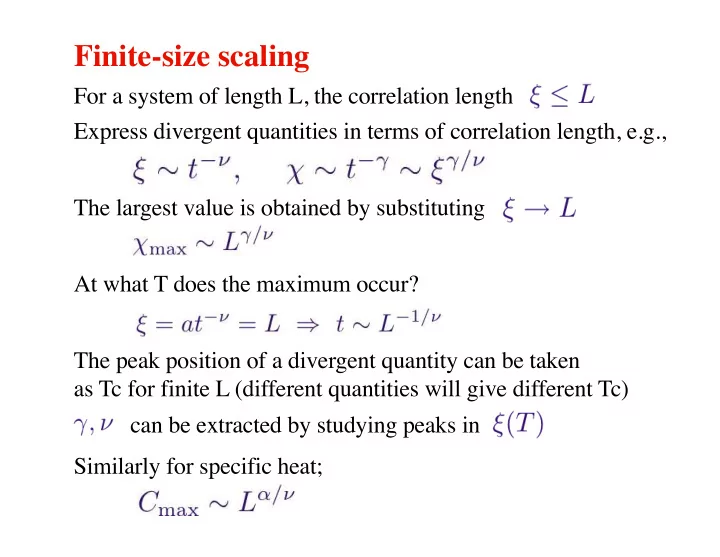
For a system of length L, the correlation length Express divergent quantities in terms of correlation length, e.g., The largest value is obtained by substituting At what T does the maximum occur? The peak position of a divergent quantity can be taken as Tc for finite L (different quantities will give different Tc) can be extracted by studying peaks in Similarly for specific heat;

SLIDE 2

Susceptibility: Diverges at the transition:

SLIDE 3

On a logarithmic scale

SLIDE 4

Specific heat (actually 𝛽=0 and log divergence for 2D Ising)

SLIDE 5

General finite-size scaling hypothesis

Test this finite-size scaling form The ratio should control the behavior

f finite-size data also close to Tc

What is the exponent σ? We know that for fixed (small) t, the infinite L form should be To reproduce this, the scaling function must have the limit We can determine the exponents as follows Hence Find g by graphing versus

SLIDE 6

2D Ising model; In general; find Tc and exponents so that large-L curves scale

SLIDE 7

Binder ratio

Useful dimensionless quantity for accurately locating Tc Infinite-size behavior: Implies finite-size scalings Hence Q should be size-independent at the critical point Q(L) curves for different L cross at Tc; often small corrections

SLIDE 8

Binder ratio: Q is size independent at Tc (useful for locating Tc)

SLIDE 9

Crossing points for, e.g., sizes L, 2L can be extrapolated to infinite L to give an accurate value for Tc

in many cases: sufficient accuracy for two large sizes

SLIDE 10

Autocorrelation functions

Value of some quantity at Monte Carlo step i: The autocorrelation function measures how a quantity becomes statistically independent from its value at previous steps Asymptotical decay (time averages) Critical slowing down At a critical point for system of length L; Q=order parameter Integerated autocorrelation time

SLIDE 11

How to calculate autocorrelation functions If we want autocorrelations for up to K MC step separations, we need to store K successive measurements of quantity Q Then, shift values after each step, add latest measurement: Accumulate time-averaged correlation functions

do t=2,k tobs(t)=tobs(t-1) enddo tobs(1)=q do t=0,k-1 acorr(t)=acorr(t)+tobs(1)*tobs(1+t) enddo

Store values in vector tobs(K); first k steps to fill the vector.

SLIDE 12

2D Ising autocorrelation functions for |M| T/J=3.0 > Tc Exponentially decaying autocorrelation function

convergent autocorrelation time

SLIDE 13

T/J = 2.269 = Tc Autocorrelation time diverges with L

SLIDE 14