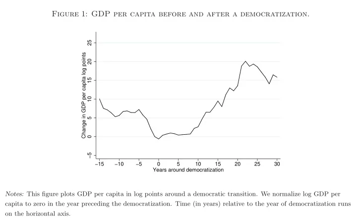
SLIDE 1 Figure 1: GDP per capita before and after a democratization.
−5 5 10 15 20 25 Change in GDP per capita log points −15 −10 −5 5 10 15 20 25 30 Years around democratization
Notes: This figure plots GDP per capita in log points around a democratic transition. We normalize log GDP per capita to zero in the year preceding the democratization. Time (in years) relative to the year of democratization runs
SLIDE 2 Table 2: Effect of democracy on (log) GDP per capita.
Within estimates Arellano and Bond estimates HHK estimates (1) (2) (3) (4) (5) (6) (7) (8) (9) (10) (11) (12) Democracy 0.973 0.651 0.787 0.887 0.959 0.797 0.875 0.659 0.781 0.582 1.178 1.682 (0.294) (0.248) (0.226) (0.245) (0.477) (0.417) (0.374) (0.378) (0.455) (0.387) (0.370) (0.352) log GDP first lag 0.973 1.266 1.238 1.233 0.946 1.216 1.204 1.204 0.938 1.158 1.150 1.155 (0.006) (0.038) (0.038) (0.039) (0.009) (0.041) (0.041) (0.038) (0.011) (0.038) (0.040) (0.036) log GDP second lag
- 0.300
- 0.207
- 0.214
- 0.270
- 0.193
- 0.205
- 0.217
- 0.127
- 0.122
(0.037) (0.046) (0.043) (0.038) (0.045) (0.042) (0.035) (0.050) (0.041) log GDP third lag
- 0.026
- 0.021
- 0.028
- 0.020
- 0.030
- 0.040
(0.028) (0.028) (0.028) (0.027) (0.026) (0.024) log GDP fourth lag
- 0.043
- 0.039
- 0.036
- 0.038
- 0.039
- 0.028
(0.017) (0.034) (0.020) (0.033) (0.015) (0.026) p-value lags 5 to 8 [ 0.565] [ 0.478] [ 0.094] Long-run effect of democracy 35.587 19.599 21.240 22.008 17.608 14.882 16.448 11.810 12.644 9.929 25.032 35.104 (13.998) (8.595) (7.215) (7.740) (10.609) (9.152) (8.436) (7.829) (8.282) (7.258) (10.581) (11.140) Effect of democracy after 25 years 17.791 13.800 16.895 17.715 13.263 12.721 14.713 10.500 10.076 8.537 20.853 29.528 (5.649) (5.550) (5.297) (5.455) (7.281) (7.371) (7.128) (6.653) (6.245) (6.032) (7.731) (7.772) Persistence of GDP process 0.973 0.967 0.963 0.960 0.946 0.946 0.947 0.944 0.938 0.941 0.953 0.952 (0.006) (0.005) (0.005) (0.007) (0.009) (0.009) (0.009) (0.009) (0.011) (0.010) (0.009) (0.009) AR2 test p-value [0.01] [0.08] [0.51] [0.95] Unit root test t−statistics
p−value (reject unit root) [0.00] [0.00] [0.00] [0.00] Observations 6,790 6,642 6,336 5,688 6,615 6,467 6,161 5,513 6,615 6,467 6,161 5,513 Countries in sample 175 175 175 175 175 175 175 175 175 175 175 175
Notes: This table presents estimates of the effect of democracy on log GDP per capita. The reported coefficient on democracy is multiplied by 100. Columns 1-4 present results using the within estimator. Columns 5-8 present results using Arellano and Bond’s GMM estimator. The AR2 row reports the p-value for a test of serial correlation in the residuals of the GDP series. Columns 9-12 present results using the HHK estimator. In all specifications we control for a full set
- f country and year fixed effects. Columns 4, 8 and 12 include 8 lags of GDP per capita as controls, but we only report the p-value of a test for joint significance
- f lags 5 to 8. Standard errors robust against heteroskedasticity and serial correlation at the country level are reported in parentheses.
SLIDE 3 Figure 2: Dynamic panel model estimates of the over-time effects of democracy on the log of GDP per capita.
10 20 30 Change in GDP per capita log points 5 10 15 20 25 30 Years around democratization
Notes: This figure plots the estimated change in the log of GDP per capita caused by a permanent transition to
- democracy. The effects are obtained by forward iteration of the estimated process for GDP modeled in equation (1). A
95% confidence interval obtained using the delta method is presented in dotted lines. Time (in years) relative to the year of democratization runs on the horizontal axis.
SLIDE 4 Table 5: Semi-parametric estimates of the effect of democratizations on (log) GDP per capita.
0 to 4 5 to 9 10 to 14 15 to 19 20 to 24 25 to 29 Average effects from: years years years years years years years (1) (2) (3) (4) (5) (6) (7) Panel A: Linear regression adjustment. Average effect of democracy on log GDP 0.060 2.454 3.621 7.806 14.037 24.075 21.310 (0.156) (1.382) (2.792) (4.416) (5.384) (8.262) (9.643) Panel B: Inverse propensity score reweighting. Average effect of democracy on log GDP
3.724 3.214 6.818 13.542 24.111 22.184 (1.478) (1.789) (3.327) (4.848) (5.892) (9.035) (11.561) Panel C: Doubly-robust estimator. Average effect of democracy on log GDP 0.051 2.795 2.969 6.966 12.947 23.691 21.793 (0.150) (1.478) (3.070) (4.354) (4.886) (7.674) (9.612)
Notes: This table presents semi-parametric estimates of the effect of a democratization on log GDP per capita over different time horizons, indicated in the column labels. We report estimates of the average effect on the treated. Panel A presents estimates using regression adjustment to compute counterfactual
- utcomes for treated countries.
Panel B presents estimates obtained via inverse propensity score reweighting. Panel C presents estimates obtained using a doubly-robust estimator, combining the regression adjustment and the inverse propensity score reweighting. Below each estimate we report robust standard errors obtained via bootstrapping.
SLIDE 5
Figure 6: Regional democratizations and reversal waves.
.1 .2 .3 .4 .5 Mean democracy −10 −5 5 10 15 20 Years around first democratization in the region Initial nondemocracies in the region Initial nondemocracies in other regions .8 .85 .9 .95 1 Mean democracy −10 −5 5 10 15 20 Years around first reversal in the region Initial democracies in the region Initial democracies in other regions Notes: These figures illustrate the existence of regional democracy waves. The top figure plots average democracy among initial nondemocracies around the first democratization in the region. For comparison it also plots average democracy among other initial nondemocracies in other regions. The bottom figure plots average democracy among initial democracies around the first reversal in the region. For comparison it also plots average democracy among other initial democracies in other regions.
SLIDE 6 Table 6: Instrumental-variables estimates of the effect of democracy on (log) GDP per capita.
GDP in 1960 Regional Regional Spatial Spatial lags quintiles× Soviet Regional GDP & unrest lag
Covariates included: year effects dummies trends trade GDP & trade
democracy (1) (2) (3) (4) (5) (6) (7) (8) (9) Panel A: 2SLS estimates with fixed effects. Democracy 0.966 1.149 1.125 1.292 1.697 1.817 1.107 1.335 1.361 (0.558) (0.554) (0.689) (0.651) (0.885) (0.663) (0.656) (0.536) (0.895) Long-run effect of democracy 26.315 31.521 35.226 35.723 36.788 41.544 25.016 37.482 38.439 (17.075) (17.425) (23.846) (19.997) (20.657) (17.157) (16.002) (17.836) (27.883) Effect of democracy after 25 years 20.836 24.866 25.618 27.929 32.051 35.350 21.386 29.217 29.011 (12.862) (12.978) (16.538) (14.944) (17.703) (14.017) (13.342) (12.894) (19.692) Persistence of GDP process 0.963 0.964 0.968 0.964 0.954 0.956 0.956 0.964 0.965 (0.005) (0.005) (0.005) (0.005) (0.006) (0.006) (0.006) (0.005) (0.006) Hansen p-value [0.21] [0.18] [0.32] [0.28] [0.25] [0.09] [0.04] [0.19] Observations 6,312 6,309 5,496 6,309 6,309 6,309 6,309 6,181 6,009 Countries in sample 174 174 148 174 174 174 174 173 173
119.1 33.2 16.8 26.7 23.7 13.6 16.7 17.5 4.6 Panel B: First-stage estimates. Democracy wave t-1 0.800 0.547 0.503 0.480 0.498 0.522 0.508 0.540 0.586 (0.073) (0.101) (0.130) (0.099) (0.092) (0.104) (0.102) (0.103) (0.101) Democracy wave t-2 0.133 0.109 0.133 0.129 0.117 0.115 0.136 0.128 (0.081) (0.094) (0.080) (0.081) (0.079) (0.078) (0.078) (0.088) Democracy wave t-3 0.227 0.270 0.223 0.228 0.221 0.223 0.224 0.282 (0.067) (0.077) (0.065) (0.070) (0.069) (0.070) (0.070) (0.077) Democracy wave t-4
- 0.087
- 0.119
- 0.075
- 0.123
- 0.083
- 0.064
- 0.072
- 0.107
(0.110) (0.126) (0.110) (0.106) (0.113) (0.113) (0.113) (0.116) Panel C: HHK estimates. Democracy 0.690 0.944 1.435 0.719 0.822 1.311 0.897 1.021 1.206 (0.642) (0.479) (0.599) (0.503) (0.480) (0.435) (0.371) (0.549) (0.485) Long-run effect of democracy 14.512 24.766 46.767 18.337 16.413 24.040 17.290 29.286 31.111 (14.703) (14.083) (22.556) (13.688) (10.700) (9.989) (8.556) (18.354) (15.167) Effect of democracy after 25 years 11.768 18.670 31.039 13.969 13.778 21.100 14.668 21.133 23.702 (11.445) (9.799) (13.113) (9.935) (8.523) (8.038) (6.734) (11.942) (10.243) Persistence of GDP process 0.952 0.962 0.969 0.961 0.950 0.945 0.948 0.965 0.961 (0.011) (0.008) (0.008) (0.009) (0.010) (0.010) (0.010) (0.009) (0.008) Observations 6,161 6,161 5,374 6,161 6,161 6,161 6,161 6,132 5,960 Countries in sample 174 174 148 174 174 174 174 173 173 Notes: This table presents IV estimates of the effect of democracy on log GDP per capita. The reported coefficient of democracy is multiplied by 100. Panel A presents 2SLS estimates instrumenting democracy with up to four lags of regional democracy waves and the p-value of a Hansen overidentification test. Panel B presents the corresponding first stage estimates and the excluded instruments F statistic. Panel C presents results using the HHK estimator instrumenting democracy with up to four lags of regional democracy waves (except for column 1, where we only use one lag). In all specifications we control for a full set of country and year fixed effects and four lags of GDP per capita. Additionally, we control for the covariates specified in each column label and described in the
- text. Standard errors robust against heteroskedasticity and serial correlation at the country level are in parentheses.
SLIDE 7 Table 8: Heterogeneous effects of democracy on (log) GDP per capita.
Interaction with: Log GDP per capita: Share with secondary: Measured at: 1960 1970 1980 Lagged 1960 1970 1980 Lagged (1) (2) (3) (4) (5) (6) (7) (8) Panel A: Within estimates. Democracy 0.432 0.572 0.687 0.744 0.446 0.340 0.385 0.495 (0.275) (0.248) (0.248) (0.246) (0.254) (0.253) (0.246) (0.241) Interaction 0.001 0.001 0.002 0.001 0.046 0.049 0.038 0.020 (0.002) (0.001) (0.002) (0.002) (0.028) (0.020) (0.014) (0.013) Long-run effect of democracy 16.231 18.631 20.489 19.843 13.785 10.480 11.841 14.597 (11.160) (9.073) (8.608) (8.255) (8.550) (8.275) (8.118) (8.432) Effect of democracy after 25 years 10.013 12.916 14.985 15.877 10.081 7.679 8.687 10.953 (6.565) (5.960) (5.848) (5.943) (5.964) (5.872) (5.728) (5.821) Persistence of GDP process 0.973 0.969 0.966 0.963 0.968 0.968 0.967 0.966 (0.005) (0.005) (0.005) (0.006) (0.005) (0.005) (0.005) (0.006) Observations 4,281 4,909 5,525 6,336 5,300 5,300 5,300 5,300 Countries in sample 93 109 131 175 138 138 138 138 Panel B: 2SLS estimates. Democracy 0.500 0.155 0.645 1.326
0.600 (1.088) (0.961) (0.929) (0.887) (0.662) (0.665) (0.639) (0.576) Interaction
0.000
0.174 0.156 0.116 0.049 (0.005) (0.004) (0.004) (0.004) (0.060) (0.047) (0.033) (0.023) Long-run effect of democracy 18.838 4.978 19.275 36.116
17.373 (43.554) (31.473) (30.208) (29.900) (19.968) (19.023) (18.114) (18.629) Effect of democracy after 25 years 11.592 3.486 14.078 28.377
13.133 (25.784) (21.795) (21.085) (21.317) (14.837) (14.524) (13.901) (13.312) Persistence of GDP process 0.973 0.969 0.967 0.963 0.967 0.967 0.966 0.965 (0.006) (0.006) (0.006) (0.008) (0.006) (0.006) (0.006) (0.006)
6.6 6.1 7.0 14.0 18.5 17.6 16.0 12.4 Hansen p-value [0.81] [0.73] [0.54] [0.33] [0.44] [0.41] [0.25] [0.50] Observations 4,273 4,901 5,517 6,153 5,292 5,292 5,292 5,218 Countries in sample 93 109 131 174 138 138 138 138 Panel C: HHK estimates. Democracy 0.222 0.234 0.144 1.619 1.101 0.887 0.790 1.713 (0.379) (0.401) (0.445) (0.477) (0.686) (0.679) (0.638) (0.584) Interaction 0.004
0.001 0.002 0.093 0.089 0.058 0.016 (0.003) (0.003) (0.004) (0.004) (0.046) (0.037) (0.028) (0.013) Long-run effect of democracy 7.692 7.453 4.480 48.375 31.605 25.022 22.375 49.338 (13.442) (13.213) (14.002) (21.975) (21.502) (20.748) (19.522) (23.950) Effect of democracy after 25 years 4.869 5.084 3.054 34.304 23.787 19.159 17.091 36.069 (8.286) (8.850) (9.435) (11.965) (15.084) (14.981) (14.107) (14.116) Persistence of GDP process 0.971 0.969 0.968 0.967 0.965 0.965 0.965 0.965 (0.009) (0.008) (0.008) (0.009) (0.008) (0.008) (0.008) (0.009) Observations 4,180 4,792 5,386 6,110 5,154 5,154 5,154 5,154 Countries in sample 93 109 131 174 138 138 138 138
Notes: This table presents estimates of the effect of democracy on log GDP per capita and its interaction with other country characteristics indicated in the columns’ headers. The reported coefficients of democracy and the interaction are multiplied by 100. We report main effects and long-run effects evaluated at the 25th percentile of the interacted variable. Panel A presents within estimates. Panel B presents 2SLS estimates instrumenting democracy (and the interaction term) with four lags of regional democracy waves. It also reports the F statistic for the excluded instruments and the p-value of Hansen’s overidentification test. Panel C presents results using the HHK estimator instrumenting democracy (and the interaction term) with four lags of regional democracy waves. In all specifications we control for a full set of country and year fixed effects and four lags of GDP per capita. Standard errors robust against heteroskedasticity and serial correlation at the country level are in parentheses.
SLIDE 8
FIGURE 3.—The spatial distribution of the Swing riots. Note: This map shows the intensity and geographic pattern of the Swing riots (August 1830–February 1831). The circles indicate the number of riots within a 10 km radius of each of the 244 English constituencies. Source: Holland (2005).
SLIDE 9 TABLE II LOCAL SWING RIOTS AND THE OUTCOME OF THE 1831 ELECTION. BASELINE RESULTSa
(1) (2) (3) (4) (5) (6)
Panel A
Whig Share 1831 (%) Least Squares
Riots within 10 km 057 037 044 047 047 044 (032)∗ (022)∗ (018)∗∗ (018)∗∗ (018)∗∗ (018)∗∗ [025]∗∗ [019]∗ [018]∗∗ [018]∗∗ [019]∗∗ [018]∗∗ Whig share 1826 087 032 035 038 038 (019)∗∗∗ (019) (020)∗ (020)∗ (0071)∗∗∗ (Whig share 1826)2 −00045 000055 000035 −68e−06 (00019)∗∗ (00020) (00020) (00020) Reform support 1830 120 121 112 121 126 (560)∗∗ (497)∗∗ (509)∗∗ (514)∗∗ (477)∗∗ County constituency 330 372 352 316 (514)∗∗∗ (650)∗∗∗ (704)∗∗∗ (468)∗∗∗ University constituency −608 −581 −581 −618 (939)∗∗∗ (107)∗∗∗ (860)∗∗∗ (1050)∗∗∗ Narrow franchise −335 −285 −362 (562) (539) (526) Patronage index −170 −135 −122 −153 (342)∗∗∗ (394)∗∗∗ (386)∗∗∗ (352)∗∗∗
752 783 (309) (2949) Agriculture (emp. share) −284 −272 (275) (270) Trade (emp. share) 114 140 (309) (311) Professionals (emp. share) −143 −119 (120) (120) Population 000028 (0009) Population density 015 (268) Thriving economy −101 (591)∗ Declining economy −106 −103 (586)∗ (572)∗ Selection ratio N.A. 067 226 254 256 259 Adjusted R2 0021 027 044 044 045 045
244 244 244 244 244 244 (Continues)
SLIDE 10 TABLE II—Continued
(1) (2) (3) (4) (5) (6)
Panel B
Whig Elected 1831 Probit
Riots within 10 km 00058 00056 00062 00068 00056 00065 [00029]∗∗ [00028]∗∗ [00029]∗∗ [00029]∗∗ [00027]∗∗ [00029]∗∗
489 489 489 489 489 489
aPanel A reports least squares estimates associating local Swing riots to the outcome of the 1831 election (constant
terms not shown). We report spatial (Conley (1999)) standard errors (50 km radius) in parentheses and White robust standard errors in brackets. The selection ratio (Altonji, Taber, and Elder (2005)) indicates how large the selection
- n unobserved factors must be relative to the selection on the observed factors included in each specification for the
point estimate on Riots within 10 km to entirely result from an omitted variables bias. The regression in column (6) is tested down using a general-to-specific approach. Panel B reports probit results (marginal effects evaluated at the mean) associating local Swing riots to the likelihood that a Whig is elected to a seat in 1831. Each estimation includes the same control variables as the corresponding estimation in panel A, except that we cannot condition on University constituency because the two university constituencies elected Tories to all four seats. The full results are reported in Table S2 in the Supplemental Material. The standard errors in panel B are clustered at the constituency level.
∗∗∗, ∗∗, and ∗ indicate statistical significance at the 1%, 5%, and 10% level, respectively.
SLIDE 11 TABLE III LOCAL SWING RIOTS AND THE OUTCOME OF THE 1831 AND 1830 ELECTIONS ALTERNATIVE MEASURES OF LOCAL SWING RIOTS AND SPATIAL CORRELATIONa
(1) (2) (3) (4) (5) (6)
Panel A
Whig Share 1831 (%) Least Squares
Riots within 1 km 276 Riots within 10 km 047 Riots within 20 km 014 Riots within 30 km 0066 Riots within 50 km 0028 Riots between 50 and 75 km 0021 Beta coefficient 011 013 012 011 011 007 Spatial std. errors, 20 km 099∗∗∗ 020∗∗ 0060∗∗ 0030∗∗ 0013∗∗ 0016 Spatial std. errors, 50 km (102)∗∗∗ (018)∗∗ (0058)∗∗ (0028)∗∗ (0013)∗∗ (0.017) Spatial std. errors, 100 km {113}∗∗ {017}∗∗∗ {0059}∗∗ {0029}∗∗ {0013}∗∗ {0.019} Spatial std. errors, 200 km [112]∗∗ [017]∗∗∗ [0061]∗∗ [0032]∗∗ [0014]∗∗ [0020] White robust std. errors [097]∗∗∗ [019]∗∗ [0058]∗∗ [0030]∗∗ [0014]∗∗ [0.017] Adjusted R2 044 045 044 044 044 043 Panel B (Placebo Test)
Whig Share 1830 (%) Least Squares
Riots within 1 km 059 Riots within 10 km 011 Riots within 20 km 0014 Riots within 30 km −00010 Riots within 50 km −00069 Riots between 50 and 75 km −0011 Beta coefficient 003 004 001 −0002 −003 −004 Spatial std. errors, 50 km (102) (011) (0042) (0025) (0010) (0011) White robust std. errors [096] [011] [0038] [0022] [0010] [0012] Adjusted R2 056 056 056 055 056 056 Difference test (p-value) 006 003 002 002 0007 N.A. Baseline controls included YES YES YES YES YES YES
244 244 244 244 244 244
aPanel A reports least squares estimates associating local Swing riots within various radiuses from the constituency
to the outcome of the 1831 election. We report spatial (Conley (1999)) standard errors for four different radiuses (20 km, 50 km, 100 km, and 200 km) and White robust standard errors. Panel B reports the corresponding results for the placebo test on the outcome of the 1830 election. The difference test is a chi-squared test where the null hypothesis is that the coefficient on the Riots within R km variable in panel A is statistically different from the corresponding coefficient in panel B (Gelman and Stern (2006)). In both panels, the controls from column (5) in Table II are included (the coefficient in column (2) in panel A is thus the coefficient from column (5) in Table II). The beta coefficients show how many standard deviations the dependent variable will change per standard deviation increase of each of the Riots within R km variables.
∗∗∗, ∗∗, and ∗ indicate statistical significance at the 1%, 5%, and 10% level, respectively.
SLIDE 12
TABLE V DISTANCE TO SEVENOAKS AND THE OUTCOME OF THE 1831 AND 1830 ELECTIONS REDUCED FORM ESTIMATESa
(1) (2) (3) (4)
Panel A
Whig Share 1831 (%) Whig Elected 1831 Least Squares Probit
Distance to Sevenoaks −189 −260 −260 −0036 Spatial std. errorsb (084)∗∗ (078)∗∗∗ (086)∗∗∗ White robust std. errors [067]∗∗∗ [081]∗∗∗ [087]∗∗∗ Clustered std. errorsc {0011}∗∗∗ Adjusted R2 003 044 043 Pseudo R2 041 Panel B (Placebo Test)
Whig Share 1830 (%) Whig Elected 1830 Least Squares Probit
Distance to Sevenoaks −084 039 046 0013 Spatial std. errorsb (060) (075) (079) White robust std. errors [057] [075] [080] Clustered std. errorsc {0014} Adjusted R2 0005 055 055 Pseudo R2 0.45 Baseline controls includedd NO YES YES YES Spatial controls includede NO YES YES YES Kent included YES YES NO YES Observations 244 244 235 489
aPanel A reports reduced form least squares and Probit estimates for the effect of Distance to Sevenoaks (the
village in Kent where the riots began) on the outcome of the 1831 election. Panel B reports the corresponding placebo estimates for the outcome of the 1830 election. In column (3), we exclude the constituencies in Kent. In column (4), the point estimate is the marginal effect which is evaluated at the mean of the explanatory variables.
bSpatial (Conley (1999)) standard errors (50 km radius). cClustered at the constituency level. dThe controls are those from column (5) in Table II. In column (4), University constituency is excluded because it
predicts the outcome perfectly as the two university constituencies elected Tories to all four seats.
eThe spatial controls are Distance to urban center, Connection to London, Market integration, Cereal area, and Dairy
area.
∗∗∗, ∗∗, and ∗ indicate statistical significance at the 1%, 5%, and 10% level, respectively.
SLIDE 13
TABLE VI LOCAL SWING RIOTS AND THE OUTCOME OF THE 1831 AND 1830 ELECTIONS INSTRUMENTAL VARIABLE ESTIMATESa
(1) (2) (3) (4)
Panel A
Whig Share 1831 (%) Whig Elected 1831 Second Stage 2SLS 2SLS 2SLS IV-Probit
Riots within 10 km (instrumented) 132 253 348 0078 Spatial GMM std. errorsb (060)∗∗ (108)∗∗ (160)∗∗ 2SLS robust std. errors [046]∗∗∗ [087]∗∗∗ [132]∗∗∗ Anderson–Rubin p-valuesg 0006 0002 0003 Clustered std. errorsc {0015}∗∗∗ Panel B
The Instrumented Variable Is Riots Within 10 km First Stage
Distance to Sevenoaks −143 −103 −075 −106 White robust std. error 017∗∗∗ 026∗∗∗ 024∗∗∗ Clustered std. errorsc {026}∗∗∗ Partial R2 on excluded instrument 023 005 003 Kleibergen–Paap F-statistic 743∗∗∗ 152∗∗∗ 99∗∗∗ Panel C
Whig Share 1831 (%) Whig Elected 1831 Least Squares Probit
Riots within 10 km 057 050 052 0.0069 Spatial std. errorsd (032)∗ (019)∗∗ (025)∗∗ White robust std. errors [025]∗∗ [021]∗∗ [029]∗ Clustered std. errorsc {00031}∗∗ (Continues)
SLIDE 14 TABLE VI—Continued
(1) (2) (3) (4)
Panel D (Placebo Test)
Whig Share 1830 (%) Whig Elected 1830 Second Stage 2SLS 2SLS 2SLS IV-Probit
Riots within 10 km (instrumented) 059 −038 −061 −0028 Spatial GMM std. errorsb (043) (075) (111) 2SLS robust std. errors [039] [071] [105] Anderson–Rubin p-valuesg 014 060 056 Clustered std. errorsc {0028} Baseline controls includede NO YES YES YES Spatial controls includedf NO YES YES YES Kent included YES YES NO YES Observations 244 244 235 489
aPanel A reports 2SLS and IV-probit estimates of the effect of local Swing riots on the outcome of the 1831
- election. Panel B, columns (1) to (3) summarize the first stage estimates for the 2SLS procedure and column (4)
summarizes the Maximum Likelihood estimates from the IV-probit procedure. Panel C reports the least squares estimates corresponding to the instrumental variable estimates in Panel A. Panel D reports the placebo second stage estimates related to the outcome of the 1830 election. The instrument is Distance to Sevenoaks (the village in Kent where the riots began). The point estimates in column (4) are marginal effects evaluated at the mean of the explanatory
- variables. The full sets of results are reported in Tables S13 to S16 in the Supplemental Material.
bSpatial (Conley (1999)) GMM standard errors (50 km radius). cClustered at the constituency level. dSpatial (Conley (1999)) standard errors (50 km radius). eThe controls are those from column (5) in Table II. In column (4), University constituency is excluded because it
predicts the outcome perfectly as the two university constituencies elected Tories to all four seats.
fThe spatial controls are Distance to urban center, Connection to London, Market integration, Cereal area, and Dairy
area.
gThe Anderson–Rubin test of significance of Riots within 10 km is robust to weak instruments. ∗∗∗, ∗∗, and ∗ indicate statistical significance at the 1%, 5%, and 10% level, respectively.