Fiberbundle-Based Visualization of a Stir Tank Fluid Benger Werner, - PowerPoint PPT Presentation

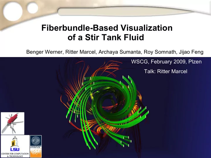
Fiberbundle-Based Visualization of a Stir Tank Fluid Benger Werner, Ritter Marcel, Archaya Sumanta, Roy Somnath, Jijao Feng WSCG, February 2009, Plzen Talk: Ritter Marcel

Outline 1.Data to be Visualized 2.Fiber Bundle Data Model ● Grid and Field Objects 3.Streamline Visualization in Vish ● Module Separation ● Using Grid Objects 4.Conclusion

1. Data to be Visualized 1/2 ● The Stirtank Dataset ● Department of Mechanical Engineering (LSU) – Sumanta Acharya – Somnath Roy ● 2088 curvilinear blocks ● Vectorfield describing velocity ● Scalarfield describing pressure

1. Data to be Visualized 2/2 ● Streamlines – Common tool to visualize vector fields such as the stirtank velocity field – Definition: (0.7, 4.3) – Simple algorithm: 3 2 Seed Point P3 1 P2 P1 0 (-1.2, 2.3) 0 1 2 3 4 5 – More complex in case of curvilinear multiblock data – What data structures should be used for the data?

2. Fiber Bundle Data Model 1/4 ● Data model based on the theory of Fiber Bundles – Identifies characteristics of scientific data – Consistent data organization – Separating Base Spaces ( Grid ) and Fibers ( Fields ) Grid (base space) data: Field (fibers) scalar values on an hexahedral curvilinear grid

2. Fiber Bundle Data Model 2/4 ● Grid object: – Manifold describing the base space – Properties: ● Topology ● Refinement level ● Coordinate representation ● Vertex positions in representation

2. Fiber Bundle Data Model 3/4 ● Internal data structure (example stirtank) – Directory structure Bundle: stirtank data Time Slice : 0.5 Grid 1: “Name1” Topology: Vertices Representation Grid 2: Cartesian XYZ “Name2” Fragmented Field Positions Representation Fragmented Field Time Slice: Cylindrical Vectors 0.6 Fragmented Field Scalars

2. Fiber Bundle Data Model 4/4 ● The user only deals with – Bundles – Grids (parameterized e.g. with time) – Fields

3. Streamline Visualization 1/6 ● Streamline-modules and Dataflow in VISH – all-in-one module solution was developed first – module separation lead to better code reusability ● Streamline-modules: – Defining seed points ● output a Grid – Compute streamlines ● input a Grid ● output a Grid – Render line grids ● input a Grid

3. Streamline Visualization 2/6 ● Defining an Input Grid for seeding streamlines – first module created point Grids on defined geometries (like points on a line or circle) – idea of copying and transforming points based on other grid points, similar to the mathematical convolution operation -> GridConvolver ( a pure Grid operation on the base space ) – led to some operations purely on Grid objects

3. Streamline Visualization 3/6 ● Gridconvolver:

3. Streamline Visualization 4/6 ● Using the Input Grid – opened the possibility to use any other Grids for seeding, such as an isosurface of pressure – without any new code development

3. Streamline Visualization 4/6 ● Using the Input Grid – opened the possibility to use any other Grids for seeding, such as an isosurface of pressure – without any new code development

3. Streamline Visualization 5/6 Streamlines seeded by isosurface of pressure helps ● to find reagons of vorticity in the velocity field Streamlines colored by magnitude ●

3. Streamline Visualization 6/6 Streamlines seeded by isosurface of pressure helps ● to find reagons of vorticity in the velocity field Streamlines colored by length ●

4. Conclusion 1/3 ● Using the software framework Vish – simplified software development by using its infrastructure and features – ensures that scientists really can use the developed modules in the 3D visualization application – see: http://sciviz.cct.lsu.edu/projects/vish/

4. Conclusion 2/3 ● Applying the Fiber Bundle Data Model for streamline visualization – revealed unexpected possibilities – made the approach very flexibly and reusable – up to now all data we encountered could be mapped into the Fiber Bundle Data Model

4. Conclusion 3/3 ● Grids used in the vish ualization: Stirtank Grid: curvilinear multiblocks Streamline Grid: hexahedral cells line grids Seeding Grid: Seeding Grid: point grid iso surface without connectivity triangular surface

End