FAULT INTERPRETATION: AUTOMATIC CURVE MATCHING Fault interpretation - - PDF document

Fault interpretation is carried out by Archimedes using an Automatic Curve Matching (ACM) method applied to located magnetic data. ACM analyses a single magnetic anomaly along a flight line or profile extracted from a gridded Total Magnetic Intensity (TMI) field in a purely automatic manner. This method works by identifying a magnetic anomaly on a profile, comparing the unique sets of components of the observed anomaly with the one that is computed for a theoretical prism, plate or edge model, varying the parameters and accepting the solution which provides the best fit.

ARCHIMEDES | THEORY

FAULT INTERPRETATION: AUTOMATIC CURVE MATCHING

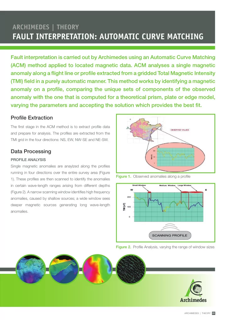
Figure 1. Observed anomalies along a profile Figure 2. Profile Analysis, varying the range of window sizes

ARCHIMEDES฀฀|฀฀THEORY฀฀฀01

Profile Extraction

The first stage in the ACM method is to extract profile data and prepare for analysis. The profiles are extracted from the TMI grid in the four directions: NS, EW, NW-SE and NE-SW.

Data Processing

PROFILE ANALYSIS Single magnetic anomalies are anaylzed along the profiles running in four directions over the entire survey area (Figure 1). These profiles are then scanned to identify the anomalies in certain wave-length ranges arising from different depths (Figure 2). A narrow scanning window identifies high frequency anomalies, caused by shallow sources; a wide window sees deeper magnetic sources generating long wave-length anomalies.

฀02

Data Processing continued

ARCHIMEDES | THEORY

FAULT INTERPRETATION: AUTOMATIC CURVE MATCHING

A series of theoretical models with different parameters capturing the variation in shape, size and magnetisation of potential magnetic bodies is prepared. Three main models are used:

• ฀ A฀ dyke-like฀ body฀ where฀ the฀ depth฀

extent is much greater than the depth to the top of the body (Figure 34); this could be used to approximate the bulk฀ volume฀ of฀ the฀ concentration฀ of฀ magnetized material.

• ฀ A฀plate฀or฀thin฀sheet฀body฀where฀the฀

depth extent is much less than the depth to the top of the body (Figure 4); this could be used to approximate sedimentary horizons, and

• ฀ An฀edge฀or฀contact฀model฀(Figure฀5);฀

this could be used to approximate geological contacts. The observed data and profiles are extracted from grids of the TMI field and are then scanned with a range of window sizes designed to detect anomalies arising from different depths. OBSERVED DATA AND MODEL DATA CORRELATION Each single anomaly (observed and theoretical) can be represented by vertical and horizontal components, which can be further split into symmetrical and asymmetrical functions. Therefore one anomaly is represented by a unique set of four

• functions. The process of comparing such a set of functions

representing the observed anomaly with the theoretical anomaly฀is฀known฀as฀‘curve฀matching’฀(Figure฀6).฀Stringent฀ similarity coefficient cut-offs (a measure of the goodness of fit of the four matched functions) are used to ensure best fjt฀ and฀ high฀ confjdence฀ results.฀ By฀ taking฀ this฀ approach฀ a฀ unique solution showing: depth, width, dip and magnetic susceptibility of the causative body is obtained. Fig 3. Fig 4. Fig 5. Figure 6. Curve matching of four components from

• bserved and theoretical data.

(b)

OUTPUT DATA The ACM technique computes depth, susceptibility, and geometry of the causative body, as well as a similarity

• coefficient. This is repeated for each model and in each profile

direction (Figure 7). The results obtained are then combined into a 3D data volume (Figure 8 The฀3D฀volume฀can฀then฀be฀taken฀into฀a฀work฀station฀where฀ the visualisation tools can be used to interpret lineaments and potential faults. FAULT INTERPRETATION The results are further analysed to identify the most statistically significant results, which are visualized in 3D. Manual interpretation is carried out, generally in the planar view of successive depth intervals panelling through the volume of the data (Figure 10). The lineaments at multiple depths can be joined vertically, that allows identification of the large scale faults in 3D. By examining various combinations of the theoretical models, as well as different directions of the profiles, structures within the sediments and the underlying basement are interpreted (Figure 9). The ability to identify faults can be affected by several factors including the extent of magnetization along the fault plane and the฀contrast฀in฀magnetic฀susceptibility฀of฀the฀rocks฀on฀either฀ side฀of฀the฀fault฀plane.฀These฀factors฀can฀make฀identifjcation฀

• f both non-mineralised and mineralised faults possible.

When the ACM results from all the profile directions supports the presence of a fault, and the lineaments can be correlated laterally and at depth, a fault plane can be gridded in 3D (Figure 10).

ARCHIMEDES฀฀|฀฀THEORY฀฀฀03

Figure 7. Depth profiles produced by curve matching Figure 8. a ‘Dots’฀and฀surfaces฀displayed฀in฀3D b Lineament interpretation along with surfaces and฀‘dots’฀displayed฀in฀3D Fig 8a Fig 8b

฀฀04฀฀ARCHIMEDES฀฀|฀฀THEORY฀฀

Summary

Archimedes approach to the interpretation of high resolution aeromagnetic data allows the detection in 3D of faults, associated structures and even fracture patterns within different sedimentary formations, as well as the underlying basement. Results are฀delivered฀in฀work฀station฀ready฀formats฀for฀integration฀with฀other฀geoscience฀data.฀Our฀proprietary฀techniques฀extract฀the฀ maximum information and deliver a detailed interpretation to aid in further exploration and development. Figure 10. Lineaments observed at different depths and interpreted as faults. Figure 9. Identification and interpretation of magnetic lineaments.

ARCHIMEDES | THEORY

FAULT INTERPRETATION: AUTOMATIC CURVE MATCHING