[PPT] - Extreme statistics of random and quantum chaotic states Steve PowerPoint Presentation

SLIDE 1

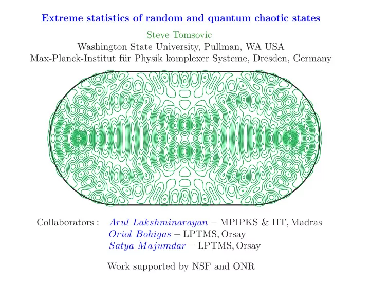
Extreme statistics of random and quantum chaotic states Steve Tomsovic Washington State University, Pullman, WA USA Max-Planck-Institut f¨ ur Physik komplexer Systeme, Dresden, Germany Collaborators : Arul Lakshminarayan − MPIPKS & IIT, Madras Oriol Bohigas − LPTMS, Orsay Satya Majumdar − LPTMS, Orsay Work supported by NSF and ONR

SLIDE 2

Today’s Thread of Logic 1) The statistics of extreme eigenstate intensities

Densities and distribution functions

Largest and smallest intensities

Universal distributions

Weibull/Fr´ echet Gumbel 2) Random states and chaotic quantum eigenstates

Complex random states and unitary ensembles1

Exact results Kicked rotor

Real random states and orthogonal ensembles

Saddle point approximations

1recent published work: A. Lakshminarayan et al., Phys. Rev. Lett. 100, 044103 (2008).

SLIDE 3

Distribution functions for maxima and minima intensities

Suppose an ensemble of systems acts in an N-dimensional vector space,{|j},

j = 1, ..., N with eigenvectors of a member system,{|φn}, n = 1, ..., N. Then, the intensities for a single eigenstate are sj = |φn|j|2

Using n and the system ensemble, a joint intensity probability density

can be defined and denoted ρ( s; N) = ρ(s1, s2, ..., sN; N)

Let the maximum intensity be s = max [sj] , j = 1, ...N
The distribution function is given by,

Fmax(t; N) = t

1 N

ds ρmax(s; N) = t d s ρ( s; N) ; d dtFmax(t; N) = ρmax(t; N)

Or for the minimum intensity s = min [sj] , j = 1, ...N

Fmin(t; N) = 1 −

1

N

t

ds ρmin(s; N) = 1 − 1

t

d s ρ( s; N)

SLIDE 4

Distribution functions for maxima and minima uncorrelated variables

Let the {sj}, j = 1, ..., N be similarly distributed independent random

variables.

A joint probability density can be defined and denoted

ρ( s; N) = ρ(s1, s2, ..., sN; N) =

N

j=1

ρ(sj; N)

The distribution function of the maximum is given by,

Fmax(t; N) = t d s ρ( s; N) = t dsj ρ(sj; N) N (any j)

Or for the minimum

Fmin(t; N) = 1 −

t

d s ρ( s; N) = 1 −

1 −

t dsj ρ(sj; N) N

SLIDE 5

Universal distribution functions - Fisher/Tippett 1928 uncorrelated variables (cont.)

The Weibull/Fr´

echet distribution function F(t; N) = 1 − exp[−(±t − aN)γN /bN] is expected for uncorrelated random variables with compact support from above or below (or heavy tailed densities).

The Gumbel distribution function

F(t; N) = exp[−e−(t−aN)/bN ] is expected for uncorrelated random variables with non-compact support whose tails decay at least exponentially fast.

For example, consider the uniform density ρ(t) = 1 (0 ≤ t ≤ 1):

Fmax(t; N) = tN − → e−N(1−t) Weibull Fmin(t; N) = 1 − (1 − t)N − → 1 − e−Nt Fr´ echet

SLIDE 6

Two relevant examples: complex and real Gaussian amplitudes uncorrelated variables (cont.)

Complex Gaussian amplitude leads to

1 N -mean intensity density:

ρ(t) = Ne−Nt (0 ≤ t ≤ ∞)

and hence

Fmax(t; N) =

1 − e−NtN

→ exp

−e−N(t− 1

N ln N)

Gumbel Fmin(t; N) = 1 −

1 −
1 − e−NtN = 1 − e−N 2t

Fr´ echet

Real Gaussian amplitude leads to

1 N -mean intensity density:

ρ(t) =

N

2πte−Nt/2 (0 ≤ t ≤ ∞)

and hence

Fmax(t; N) = erfN Nt/2

→ exp
−e− N

2 (t− 1 N ln 2N πt )

Gumbel? Fmin(t; N) = 1 −

1 − erf
Nt/2

N → 1 − e−

q

2N3t π

Fr´ echet

SLIDE 7

Joint probability densities for intensities correlated variables

A norm constraint is naturally expressed in amplitude variables:

ρβ(z1, z2, . . . , zN) = Γ

Nβ

2

πNβ/2

δ  

N

j=1

|zj|2 − 1   where β = 1, 2 for real and complex respectively. The real case corre- sponds to the orthogonal random matrix ensembles and the complex case to the unitary ensembles. Switching to intensities: ρβ( s; N) = πN(β/2−1)Γ Nβ 2  

N

j=1

sβ/2−1

j

dsj   δ  

N

j=1

sj − 1  

The complex case is equivalent to the “broken stick problem” in which

N −1 cuts at uniformly random locations are made in a unit length stick.

The real case is intimately connected to the relationship between hyper-

spherical and cartesian coordinates.

SLIDE 8

An auxiliary function for “decorrelating” intensities

The distribution function for the maximum is:

F β

max(t; N) = πN(β/2−1)Γ

Nβ 2  

N

j=1

t sβ/2−1

j

dsj   δ  

N

j=1

sj − 1  

Define the auxiliary function Gβ(t, u; N) which results from replacing

unity in the norm constraint by u and thus, F β

max(t; N) = Gβ(t, u = 1; N).

The Laplace transform of Gβ(t, u; N) renders the integrals over the N

differentials dsj into a product form and gives: ∞ e−usGβ(t, N, u)du =      Γ( N

2 )

erf(

√ st) √s

N real Γ(N)

1−e−st

s

N complex

The N integrals have been performed at the cost of now needing the

inverse Laplace transforms of these expressions.

SLIDE 9

Exact results for unitary ensembles

The distribution function for the maximum follows by expanding the N th

power and using the inverse Laplace transform: L−1

s

e−smt sN

=

1 Γ(N)(u − mt)N−1Θ(u − mt) and gives F β=2

max(t; N) = N

m=0

N m

(−1)m(1 − mt)N−1Θ(1 − mt)
Interestingly, this reduces to a piecewise smooth expression with the in-

tervals Ik = [1/(k + 1), 1/k], where k = 1, 2, · · · , N − 1 Fmax(t ∈ Ik; N) =

k

m=0

N m

(−1)m(1 − mt)N−1
All distributions resulting from correlated variables possessing at least

unit norm constraints, satisfy a combinatoric form of this type.

SLIDE 10

Exact results for unitary ensembles (cont.)

0.0 0.2 0.4 0.6

2

2 4

ρ(x;N)

x

N=8 N=16 N=32 N=64 Gumbel

3
1

1 3 0.1 0.2 0.3 0.4 0.5

t

The exact probability density and the asymptotic Gumbel density using the scaled variable x = N(t − ln(N)/N) with increasing N. The inset shows the difference between the exact and the Gumbel densities for the same values of N, but in the unscaled variable.

SLIDE 11

The quantum kicked rotor as an example of a chaotic system 0.2 0.4

2

2 4

ρ(x;N)

x=Nt-ln N

0.2 0.4 0.6 0.8 2 4

x= N2 t maximum minimum

The probability densities (histograms) of the scaled maximum and minimum (inset) intensity of eigenfunctions in the position basis of the quantum kicked rotor for N = 32 in the parameter range 13.8 < K < 14.8. Shown as a continuous line is the exact density for random states while the dotted ones are the respective Gumbel and Fr´ echet densities.

SLIDE 12

A saddle point approximation for the orthogonal ensembles A saddle point approximation for the inverse Laplace transform: L−1

s

(πst)m/2 emsterfcm(

√ st) 1

πt

m/2 e−smt s

N+m 2

≈
N+m

2−2mt

m/2 × exp

m(N+m)t

2−2mt

erfcm
(N+m)t

2−2mt

1

Γ N+m

2

(1 − mt)

N+m 2

−1Θ(1 − mt)

gives F β=1

max(t; N) = k

m=0

N

m

(−1)m N+m

2

m

2 Γ

N

2

(1 − mt)

N 2 −1

Γ N+m

2

exp
m

N+m

2

t

1 − mt

erfcm

  N+m

2

t

1 − mt  

r more simply using only the asymptotic form of erfc(z),

F β=1

max(t; N) = k

m=0

N m

(−1)m

Γ N

2

Γ

N+m

2

(1 − mt)

N+m 2

−1

(πt)

m 2

SLIDE 13

0.2

0.2 0.4 0.6 0.8 1 0.2 0.4 0.6 0.8 1 saddle point approximation simulation

N=10 t F(t;N) The orthogonal ensembles

Gumbel distribution saddle point w/o erfc

Comparison of the maximum intensity distribution functions for the orthogonal

ensembles. The saddle point approximation improves considerably the agree-

ment with the “exact” result from simulation vis-a-vis the asymptotic Gumbel

form. The simpler form without the complementary error function is an im-

provement, but not good enough for small N to warrant its use.

SLIDE 14

Concluding remarks

The statistical properties of extreme intensities has not previously been

applied to understanding better the eigenstates of quantum systems.

It is possible to derive some compact, exact results for the unitary ensem-

bles with any dimensionality and give excellent approximations for the same quantities in the orthogonal ensemble.

The maximum intensities tend to the infinite dimensional limit very slowly

and thus the functional forms contain some information about system size. They further tend toward the Gumbel distribution although, a priori, one might have expected Weibull. Means scale as ln aβN/N for unitary and (roughly for) orthogonal ensembles.

The minimum intensity statistics tend much more rapidly toward their

infinite dimensional Fr´ echet limiting form. The mean minima are N −2 and πN −3 for the unitary and orthogonal ensembles respectively.

These “extreme” measures give us a new way to explore non-ergodic eigen-

state behaviors. – It would be worthwhile exploring: i) other measures such as the intensity densities in the neighborhood of the maxima or minima, and ii) how system dynamics lead to deviations from the chaotic statistical extremes.