Extending a 2 k design The 2 k factorial design can detect main - - PowerPoint PPT Presentation

ST 516 Experimental Statistics for Engineers II

Extending a 2k design

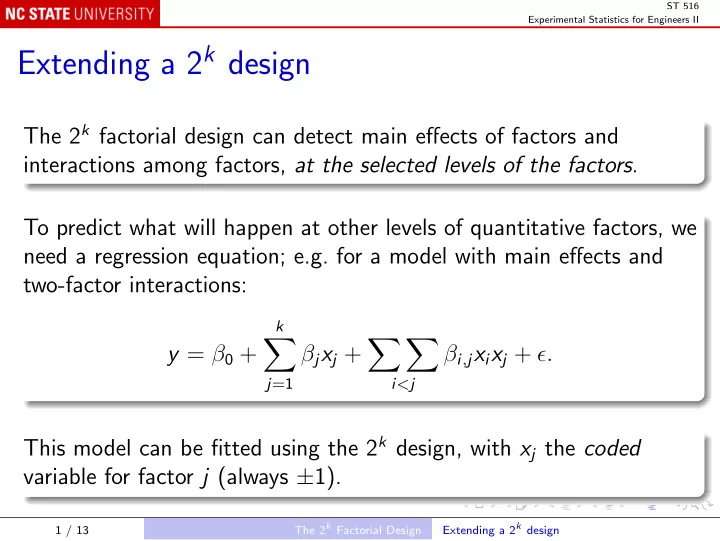
The 2k factorial design can detect main effects of factors and interactions among factors, at the selected levels of the factors. To predict what will happen at other levels of quantitative factors, we need a regression equation; e.g. for a model with main effects and two-factor interactions: y = β0 +

k

• j=1

βjxj +

i<j

βi,jxixj + ǫ. This model can be fitted using the 2k design, with xj the coded variable for factor j (always ±1).

1 / 13 The 2k Factorial Design Extending a 2k design

ST 516 Experimental Statistics for Engineers II

But: the model is linear in each xj with the other factors held fixed. Cannot detect curvature, e.g. if the true dependence is y = β0 +

k

• j=1

βjxj +

i<j

βi,jxixj +

k

• j=1

βj,jx2

j + ǫ.

In this case, extra design points are needed. E.g. if all factors are quantitative, nC runs at the center point x1 = x2 = · · · = xk = 0.

2 / 13 The 2k Factorial Design Extending a 2k design

ST 516 Experimental Statistics for Engineers II

At the original (2k factorial) design points, all x2

j = 1, so

y =

• β0 +

k

• j=1

βj,j

• +

k

• j=1

βjxj +

i<j

βi,jxixj + ǫ. So ¯ yF, the average y at the original design points, estimates β0 + k

j=1 βj,j.

But clearly ¯ yC, the average y at the center point, estimates β0.

3 / 13 The 2k Factorial Design Extending a 2k design

ST 516 Experimental Statistics for Engineers II

So we can use ¯ yF − ¯ yC to test the hypothesis H0 : βj,j = 0. This will usually detect quadratic terms (but the test has no power if βj,j = 0). Test statistic is based on SSPure quadratic = nFnC (¯ yF − ¯ yC)2 nF + nC , where nF is the number of points in the original factorial design. Replicated center values provide nC − 1 degrees of freedom to estimate σ2 (“pure error”).

4 / 13 The 2k Factorial Design Extending a 2k design

ST 516 Experimental Statistics for Engineers II

Example Filtration rate, with 4 center points (rates 73, 75, 66, 69) R code

filt2 <- read.table("data/filtration-with-center.txt", header = TRUE) summary(aov(Rate ~ A * B * C * D + I(A^2) + I(B^2) + I(C^2) + I(D^2), filt2)) summary(aov(Rate ~ A * C + A * D + I(A^2) + I(C^2) + I(D^2), filt2))

The formulas include all squared variables, but, with this design, only

• ne can be estimated.

5 / 13 The 2k Factorial Design Extending a 2k design

ST 516 Experimental Statistics for Engineers II

Full model

Df Sum Sq Mean Sq F value Pr(>F) A 1 1870.56 1870.56 115.1115 0.001731 ** B 1 39.06 39.06 2.4038 0.218821 C 1 390.06 390.06 24.0038 0.016273 * D 1 855.56 855.56 52.6500 0.005401 ** I(A^2) 1 1.51 1.51 0.0931 0.780243 A:B 1 0.06 0.06 0.0038 0.954450 A:C 1 1314.06 1314.06 80.8654 0.002903 ** B:C 1 22.56 22.56 1.3885 0.323620 A:D 1 1105.56 1105.56 68.0346 0.003731 ** B:D 1 0.56 0.56 0.0346 0.864273 C:D 1 5.06 5.06 0.3115 0.615686 A:B:C 1 14.06 14.06 0.8654 0.420856 A:B:D 1 68.06 68.06 4.1885 0.133202 A:C:D 1 10.56 10.56 0.6500 0.479099 B:C:D 1 27.56 27.56 1.6962 0.283757 A:B:C:D 1 7.56 7.56 0.4654 0.544069 Residuals 3 48.75 16.25

• Signif. codes:

0 *** 0.001 ** 0.01 * 0.05 . 0.1 1

6 / 13 The 2k Factorial Design Extending a 2k design

ST 516 Experimental Statistics for Engineers II

Reduced model

Df Sum Sq Mean Sq F value Pr(>F) A 1 1870.56 1870.56 99.7122 1.830e-07 *** C 1 390.06 390.06 20.7927 0.0005354 *** D 1 855.56 855.56 45.6066 1.356e-05 *** I(A^2) 1 1.51 1.51 0.0806 0.7809238 A:C 1 1314.06 1314.06 70.0474 1.359e-06 *** A:D 1 1105.56 1105.56 58.9331 3.502e-06 *** Residuals 13 243.88 18.76

• Signif. codes:

0 *** 0.001 ** 0.01 * 0.05 . 0.1 1

7 / 13 The 2k Factorial Design Extending a 2k design

ST 516 Experimental Statistics for Engineers II

The “Residuals” line in the reduced model may be decomposed into “Lack of Fit” and “Pure Error”:

summary(aov(Rate ~ A * C + A * D + I(A^2) + I(C^2) + I(D^2) + factor(A):factor(B):factor(C):factor(D), filt2))

Output

Df Sum Sq Mean Sq F value Pr(>F) A 1 1870.56 1870.56 115.1115 0.001731 ** C 1 390.06 390.06 24.0038 0.016273 * D 1 855.56 855.56 52.6500 0.005401 ** I(A^2) 1 1.51 1.51 0.0931 0.780243 A:C 1 1314.06 1314.06 80.8654 0.002903 ** A:D 1 1105.56 1105.56 68.0346 0.003731 ** factor(A):factor(B):factor(C):factor(D) 10 195.13 19.51 1.2008 0.494185 Residuals 3 48.75 16.25

• Signif. codes:

0 *** 0.001 ** 0.01 * 0.05 . 0.1 1

8 / 13 The 2k Factorial Design Extending a 2k design

ST 516 Experimental Statistics for Engineers II

The line for factor(A):factor(B):factor(C):factor(D) is Lack of Fit, with 10 d.f. pooled from the omitted terms. The residuals line is now Pure Error, with the 3 d.f. from the 4 center point runs.

9 / 13 The 2k Factorial Design Extending a 2k design

ST 516 Experimental Statistics for Engineers II

Central Composite Design

Adding center points allows you to detect pure quadratic terms, but not to estimate them. Need to add more points; e.g. axial points: x1 = ±α, x2 = · · · = xk = 0, x1 = 0, x2 = ±α, x3 = · · · = xk = 0, and so on; 2k extra points when unreplicated (usual case). Choice of α (nF = number of factorial runs): α = 1 convenient, as it brings in no new levels; α =

4

√nF gives desirable property (rotatability).

10 / 13 The 2k Factorial Design Extending a 2k design

ST 516 Experimental Statistics for Engineers II

Center Points with Qualitative Factors

For a qualitative factor (e.g. equipment from two suppliers), x = 0 is infeasible. Use two center points, one each at the high and low levels of the qualitative factor. Same as axial points with α = 1, but usually replicated.

11 / 13 The 2k Factorial Design Extending a 2k design

ST 516 Experimental Statistics for Engineers II

Coded Variables and Engineering Units

A quantitative factor x∗ has levels x∗

− and x∗ +.

The coded variable is x = x∗ − 1

2

• x∗

+ + x∗ −

• 1

2 (x∗ + − x∗ −)

. Regression equation in coded variables can be converted to engineering units for later use, e.g in predicting the response for arbitrary levels.

12 / 13 The 2k Factorial Design Extending a 2k design

ST 516 Experimental Statistics for Engineers II

The same equation results from fitting directly to the original factor levels. Coded variable form is useful for the experimenter: Gives all effects and interactions; The t-statistics are equivalent to F-statistics in the ANOVA table. Engineering units form is useful for others: Does not depend on experimental levels of factors; Coefficients have a different interpretation: a regression coefficient represents the effect of changing a factor by 1 (engineering) unit, not the effect of changing from low level to high level (actually, one-half that effect).

13 / 13 The 2k Factorial Design Extending a 2k design