Exponential Varieties Bernd Sturmfels UC Berkeley Joint paper with - PowerPoint PPT Presentation

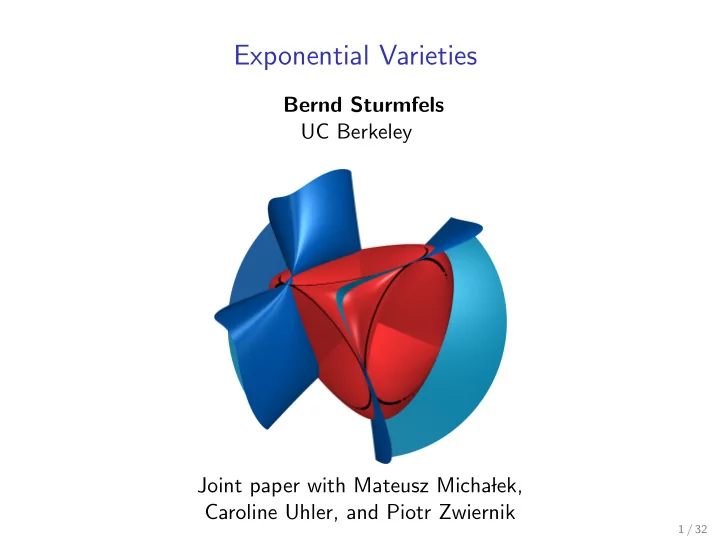
Exponential Varieties Bernd Sturmfels UC Berkeley Joint paper with Mateusz Micha� lek, Caroline Uhler, and Piotr Zwiernik 1 / 32

Motivation 1: Toric Geometry A central theme in Algebraic Statistics is the connection between toric varieties and discrete exponential families. Binomial equations defining toric varieties are Markov bases. [Diaconis-St 1998] Example (Independence of binary random variables) The Segre variety V = P 1 × P 1 ⊂ P 3 is defined by � p 00 � p 01 det = 0 . p 10 p 11 The moment map takes V onto K = the square = ∆ 1 × ∆ 1 . It computes sufficient statistics : V ≥ 0 − → K This is invertible. Its inverse is the maximum likelihood estimator . 2 / 32

Motivation 2: Gaussian Geometry Let L be a linear space of real symmetric m × m -matrices. [St-Uhler 2010] studied the variety σ ∈ Sym 2 R m : σ − 1 ∈ L � cl L − 1 � = The Gaussian model is the subset of covariance matrices σ ∈ L − 1 : σ positive definite L − 1 � � = ≻ 0 Example (Graphical models) L encodes sparsity of an undirected graph with m nodes. → Sym 2 R m computes sufficient statistics : The map dual to L ֒ L − 1 → K = ( L ≻ 0 ) ∨ . ≻ 0 − This is invertible. Its inverse is the maximum likelihood estimator . 3 / 32

Exponential Families An exponential family is a parametric statistical model � � p θ ( x ) = exp − � θ, T ( x ) � − A ( θ ) . on a sample space ( X , ν, T ), with T : X → R d measurable. Here A ( θ ) is the log-partition function . � Since X p θ ( x ) ν ( dx ) = 1, � � � A ( θ ) = log exp −� θ, T ( x ) � ν ( dx ) . X 4 / 32

Exponential Families An exponential family is a parametric statistical model � � p θ ( x ) = exp − � θ, T ( x ) � − A ( θ ) . on a sample space ( X , ν, T ), with T : X → R d measurable. Here A ( θ ) is the log-partition function . � Since X p θ ( x ) ν ( dx ) = 1, � � � A ( θ ) = log exp −� θ, T ( x ) � ν ( dx ) . X The following sets are convex : θ ∈ R d : A ( θ ) < + ∞ � � Space of canonical parameters: C = � � ⊂ R d Space of sufficient statistics: K = conv T ( X ) 5 / 32

Exponential Families An exponential family is a parametric statistical model � � p θ ( x ) = exp − � θ, T ( x ) � − A ( θ ) . on a sample space ( X , ν, T ), with T : X → R d measurable. Here A ( θ ) is the log-partition function . � Since X p θ ( x ) ν ( dx ) = 1, � � � A ( θ ) = log exp −� θ, T ( x ) � ν ( dx ) . X The following sets are convex : θ ∈ R d : A ( θ ) < + ∞ � � Space of canonical parameters: C = � � ⊂ R d Space of sufficient statistics: K = conv T ( X ) Theorem Suppose C is open and K spans R d . The gradient map F : R d → R d , θ �→ −∇ A ( θ ) defines an analytic bijection between C and int ( K ) . 6 / 32

From Analysis to Algebra Our exponential families satisfy A ( θ ) = − α · log ( f ( θ )) , where f ( θ ) is a homogeneous polynomial and α > 0. The gradient of the log-partition function is the rational function � ∂ f α , ∂ f , . . . , ∂ f R d ��� R d : θ �→ � F : f ( θ ) · . ∂θ 1 ∂θ 2 ∂θ d Algebraic geometers prefer � ∂ f : ∂ f : · · · : ∂ f F : CP d − 1 ��� CP d − 1 : θ �→ � . ∂θ 1 ∂θ 2 ∂θ d The partition function f ( θ ) α admits a nice integral representation. Which polynomials f ( θ ) and convex sets C , K ⊂ R d are possible? 7 / 32

Duality of Polytopes Example (How to morph a cube into an octahedron?) [St-Uhler 2010, Example 3.5] 8 / 32

Duality of Polytopes Example (Exponential family for cube → octahedron) Fix the product of linear forms f ( θ ) = ( θ 2 1 − θ 2 4 )( θ 2 2 − θ 2 4 )( θ 2 3 − θ 2 4 ) The space of canonical parameters is � � C = cone over the 3-cube | θ i | < 1 : i = 1 , 2 , 3 The space of sufficient statistics is K = cone over the octahedron conv {± e 1 , ± e 2 , ± e 3 } Gradient map ∇ f : P 3 ��� P 3 gives bijection between C and int ( K ). Its inverse is an algebraic function of degree 7. Question: What is ( X , ν, T ) in this case? 9 / 32

Duality of Polytopes Example (Exponential family for cube → octahedron) Fix the product of linear forms f ( θ ) = ( θ 2 1 − θ 2 4 )( θ 2 2 − θ 2 4 )( θ 2 3 − θ 2 4 ) The space of canonical parameters is � � C = cone over the 3-cube | θ i | < 1 : i = 1 , 2 , 3 The space of sufficient statistics is K = cone over the octahedron conv {± e 1 , ± e 2 , ± e 3 } Gradient map ∇ f : P 3 ��� P 3 gives bijection between C and int ( K ). Its inverse is an algebraic function of degree 7. Question: What is ( X , ν, T ) in this case? Answer: X = K , T = id , and ν constructed via hypergeometric functions 10 / 32

Hyperbolic Polynomials A homog. polynomial f ∈ R [ θ 1 , . . . , θ d ] of degree k is hyperbolic if, for some t ∈ R d , every line through t intersects the complex hypersurface { f = 0 } in k real points. The connected component C of t in R d \{ f = 0 } is the hyperbolicity cone . It is convex. 11 / 32

Hyperbolic Polynomials A homog. polynomial f ∈ R [ θ 1 , . . . , θ d ] of degree k is hyperbolic if, for some t ∈ R d , every line through t intersects the complex hypersurface { f = 0 } in k real points. The connected component C of t in R d \{ f = 0 } is the hyperbolicity cone . It is convex. Our integral representation lives on the dual hyperbolicity cone : Theorem (G˚ arding 1951 ... Scott-Sokal 2015) If α > d, there exists a measure ν on the cone K = C ∨ such that � f ( θ ) − α = exp( −� θ, σ � ) ν ( d σ ) for all θ ∈ C. K Furthermore, this property characterizes hyperbolic polynomials. 12 / 32

Hyperbolic Polynomials A homog. polynomial f ∈ R [ θ 1 , . . . , θ d ] of degree k is hyperbolic if, for some t ∈ R d , every line through t intersects the complex hypersurface { f = 0 } in k real points. The connected component C of t in R d \{ f = 0 } is the hyperbolicity cone . It is convex. Our integral representation lives on the dual hyperbolicity cone : Theorem (G˚ arding 1951 ... Scott-Sokal 2015) If α > d, there exists a measure ν on the cone K = C ∨ such that � f ( θ ) − α = exp( −� θ, σ � ) ν ( d σ ) for all θ ∈ C. K Furthermore, this property characterizes hyperbolic polynomials. Proof : Riesz kernels and more. Lots of analysis. The resulting statistical models are hyperbolic exponential families . Related to hyperbolic programming in convex optimization [G¨ uler]. 13 / 32

Hyperbolic Exponential Families: An Example The space of canonical parameters C is the hyperbolicity cone of f = θ 1 θ 2 θ 3 + θ 1 θ 2 θ 4 + θ 1 θ 3 θ 4 + θ 2 θ 3 θ 4 . 14 / 32

Its dual K = C ∨ is the space of sufficient statistics: Steiner surface a.k.a Roman surface � σ 4 � σ 3 � σ 2 i σ 2 � σ 2 i − 4 i σ j σ k − 40 σ 1 σ 2 σ 3 σ 4 . i σ j + 6 j + 4 15 / 32

Duality Gradient map ∇ f : P 3 → P 3 gives a bijection between C and K : We shall be interested in the geometry its graph X f ⊂ P 3 × P 3 . 16 / 32

Gaussian Family is Hyperbolic Let X = R m , where ν is Lebesgue measure, and set T ( x ) = 1 2 x · x T ∈ Sym 2 ( R m ) ≃ R d . The symmetric determinant f ( θ ) = det ( θ ) is a hyperbolic � m +1 � polynomial in d = unknowns. Its hyperbolicity cone C 2 consists of positive definite matrices. This cone is self-dual: K = C ∨ = conv ( T ( X )) ≃ C . 17 / 32

Gaussian Family is Hyperbolic Let X = R m , where ν is Lebesgue measure, and set T ( x ) = 1 2 x · x T ∈ Sym 2 ( R m ) ≃ R d . The symmetric determinant f ( θ ) = det ( θ ) is a hyperbolic � m +1 � polynomial in d = unknowns. Its hyperbolicity cone C 2 consists of positive definite matrices. This cone is self-dual: K = C ∨ = conv ( T ( X )) ≃ C . Integral for p θ ( x ) is the standard multivariate Gaussian, with A ( θ ) = − 1 2 log det( θ ) + m 2 log(2 π ) . The gradient map is matrix inversion F : C → K , θ �→ 1 2 θ − 1 . The measure that represents f ( θ ) − 1 / 2 comes from the Wishart distribution , i.e. the distribution of the sample covariance matrix ... 18 / 32

Intersecting with a Subspace Fix exponential family with rational gradient map F : C → K . Main case: F = ∇ f where f is hyperbolic Consider a linear subspace L ⊂ R d with C L := L ∩ C nonempty: 19 / 32

Exponential Varieties The exponential variety is the image under the gradient map: L F := F ( L ) ⊂ P d − 1 . Its positive part L F ≻ 0 lives in K . 20 / 32

Convexity and Positivity Theorem Let ( X , ν, T ) be an exponential family with rational gradient map F : R d ��� R d , and L ⊂ R d a linear subspace. The restricted gradient map F L is the composition π L F C L ⊂ C − → K − → K L . The convex set C L of canonical parameters maps bijectively to the positive exponential variety L F ≻ 0 , and L F ≻ 0 maps bijectively to the interior of the convex set K L of sufficient statistics. Maximum Likelihood Estimation for an exponential variety means inverting these two bijections, by solving polynomials. Math question: What is the algebraic degree of this inversion? 21 / 32

Bijections in Pictures Green maps to blue maps to green ∨ . Inverting this map is MLE. - 22 / 32 10