Example: Bayes rule A drug test proposed by a company tests positive - PowerPoint PPT Presentation

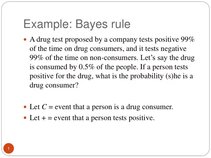
Example: Bayes rule  A drug test proposed by a company tests positive 99% of the time on drug consumers, and it tests negative 99% of the time on non- consumers. Let’s say the drug is consumed by 0.5% of the people. If a person tests positive for the drug, what is the probability (s)he is a drug consumer?  Let C = event that a person is a drug consumer.  Let + = event that a person tests positive. 1

Example: the false positive paradox   c ( ) 0 . 005 , ( ) 0 . 995 P C P C   ( | ) 0 . 99 P C     ( | ) ( | ) ( ) / ( ) P C P C P C P      c c ( ) ( | ) ( ) ( | ) ( ) P P C P C P C P C    0 . 99 * 0 . 005 ( 1 0 . 99 ) * 0 . 995 0 . 99 * 0 . 005    ( | ) 33 . 22 % P C  0 . 99 * 0 . 005 0 . 01 * 0 . 995 An individual testing positive is most likely not a consumer – despite the apparent (99%) accuracy of the test! This is because the number of drug consumers is small and hence the factor 0.995 outweighs the consumer probability! This is called the false positive paradox. For fewer false positives, we need more than 99% accuracy on non-consumers (Eg: 99.99%). More such examples on wikipedia. 2

The Birthday Paradox!  Given n people in a room, what should be the least value of n such that the probability that at least 2 people in the room share the same birthday is 99.9%?  Each person can have his/her birthday on any of the 365 days. For n people, there are 365 n outcomes.  The number of outcomes resulting in no two people sharing a birthday is (365)(364)(363)…(365 - n +1). 3

The Birthday Paradox!  So required probability is 1-(365 )(364)(363)…(365 - n +1)/(365) n = 0.999 (given)  This is satisfied for n as small as 70.  For n = 20, it is around 41%.  For n = 40, it is around 89%.  For more information see the wikipedia article on the birthday paradox. 4

Random Variables Fall 2017 Instructor: Ajit Rajwade 5

Topic Overview  Random variable: definition  Discrete and continuous random variables  Probability density function (pdf) and cumulative distribution function (cdf)  Joint and conditional pdfs  Expectation and its properties  Variance and covariance  Markov’s and Chebyshev’s inequality  Weak law of large numbers  Moment generating functions 6

Random variable  In many random experiments, we are not always interested in the observed values, but in some numerical quantity determined by the observed values.  Example: we may be interested in the sum of the values of two dice throws, or the number of heads appearing in n consecutive coin tosses.  Any such quantities determined by the results of random experiments are called as random variables (they may also be the observations themselves). 7

Random variable Value of X (Denoted P( X = x ) This is called the probability as x ) where X = sum mass function (pmf) table of of 2 dice throws the random variable X . If S is 2 1/36 the sample space, then P( S ) = P(union of all events of 3 2/36 the form X = x ) = 1 (verify 4 3/36 from table). 5 4/36 6 5/36 7 6/36 8 5/36 9 4/36 10 3/36 11 2/36 12 1/36 8

Random variable: Notation  A random variable is usually denoted by an upper case alphabet.  Individual values the random variable can acquire are denoted by lower case . 9

Random variable: discrete  Random variables whose values can be written as a finite or infinite sequence are called discrete random variables .  Example: results of coin toss or random dice experiments  The probability that a random variable X takes on value x , i.e. P( X = x ), is called as the probability mass function . 10

Random variable: continuous  Random variables that can take on values within a continuum are called continuous random variables .  Example: the dimensions (length, height, width, weight) of an object are usually continuous quantities, direction of a vector, amount of water that can be stored in a 4 litre jar is a continuous random variable in the interval [0,4]. 0 1 4 11

Random variable: continuous  For a continuous random variable, the probability that it takes on any particular value within a continuum is zero !  Why? Because there are infinitely many values – say in the interval [0,4] in the example on the previous slide. Each value will be equally likely.  Note : Zero probability in case of continuous random variables does not mean the event will never occur! This differs from the discrete case. 12

Random variable: continuous  Hence for a continuous random variable X , we consider the cumulative distribution function (cdf) F X ( x ) defined as P{ X ≤ x }.  The cdf is basically the probability that X takes on a value less than or equal to x .  The cdf can be used to compute cumulative interval measures , that is the probability that X takes on a value greater than a and less than or equal to b , i.e. P( a < X ≤ b ) = F X ( b ) -F X ( a ) . 13

Random variable: continuous - example  Consider a cdf of the form: F X ( x ) = 0 for x ≤ 0, and F X ( x ) = 1-exp(- x 2 ) otherwise  To find: probability that X exceeds 1  P( X > 1) = 1-P( X ≤1)=1 -F X (1) = e -1 14

Probability Density Function (pdf)  The pdf of a random variable X at a value x is the derivative of its cumulative distribution function (cdf) at that value x .  It is a non-negative function f X ( x ) such that for any set  B of real numbers, we have   { } ( ) P X B f x dx X B    ( ) 1 f x dx X    Properties: b       ( ) ( ) ( ) ( ) P a X b f x dx F b F a X X X a a     ( ) ( ) 0 P X a f x dx X 15 a

f X ( x ) dx a b x The area beneath the blue curve in between the lines x = a and x = b is the cumulative interval measure P( a < X ≤ b ) = F X ( b ) -F X ( a ) . f X ( a ) dx = probability that the random variable X takes on values between a and a + dx . 16

Probability Density Function  Another way of looking at this concept:   / 2 a            { / 2 / 2 } ( ) ( ) P a X a f x dx f a X  / 2 a       { / 2 / 2 } P a X a  ( ) lim f a    0 X 17

Examples: Popular families of PDFs 1     2  2 ( ) /( 2 ) x  Gaussian (normal) pdf: ( ) f x e   X 2 18

Examples: Popular families of PDFs 1    ( ) , f X x a x b   Bounded uniform pdf: ( ) b a  0 otherwise 19

Expected Value (Expectation) of a random variable  It is also called the mean value of the random variable.  For a discrete random variable X , it is defined as:    ( ) ( ) E X x P X x i i i  For a continuous random variable X , it is defined as:    ( ) ( ) E X xf x dx X    The expected value should not be (mis)interpreted to be the value that X usually takes on – it’s the average value, not the “most frequently occurring value”. 20

Expected Value (Expectation) of a random variable  For some pdfs, the expected value is not always defined, i.e. the integral below may not have a finite value.    ( ) ( ) E X xf x dx X    One example is the pdf for the Pareto distribution (under some parameters) given as:   x m and α are parameters x    ( | , ) m for , otherwise 0 f x x x x   of the pdf for the Pareto X m m 1 x distribution. Verify this      1 x  result for E( X ) on your         ( ) if 1 E X x     m  1  own. x m 21

Expected Value (Expectation) of a random variable  Likewise for some discrete random variables which take on infinitely many values, the expected value may not be defined, i.e. we may have      ( ) ( ) E X x P X x i i i  Example:      2 ( ) / for 1 , P X x k x x x Z          ( ) ( ) 1 / See here. E X xP X x k x   1 1 x x          2 2 Note : ( ) / 1 if 6 / P X x k x k See here.   1 1 x x 22

Expected Value: examples  The expected value that shows up when you throw a die is 1/6(1+2+3+4+5+6) = 3.5.  The game of roulette consists of a ball and wheel with 38 numbered pockets on its side. The ball rolls and settles on one of the pockets. If the number in the pocket is the same as the one you guessed, you win $35 (probability 1/38), otherwise you lose $1 (probability 37/38). The expected value of the amount you earn after one trial is: (-1)37/38 +(35)1/38 = $-0.0526 23

A Game of Roulette https://en.wikipedia.org/wiki/Roulette#/media/File:Roulette_casino.JPG 24

Expected value of a function of random variable  Consider a function g ( X ) of a discrete random variable X. The expected value of g ( X ) is defined as:    ( ( )) ( ) ( ) E g X g x P X x i i i  For a continuous random variable, the expected value of g ( X ) is defined as:    ( ( )) ( ) ( ) E g X g x f x dx X   25