SLIDE 38 » Summary » Heavy-tailed distributions » Characterizing Heavy-tail behavior » Π-variation and Γ-variation » A step towards estimation » Estimation of the tail parameter » Auxiliary results I » Auxiliary results II » Asymptotic normality » Main result » Finite sample behavior I » Finite sample behavior II » Finite sample behavior III » Drawback... » Test of hypothesis » Empirical power » Estimated type I error » References Cláudia Neves, August 18, 2005 EVA - p. 13/19
Finite sample behavior II
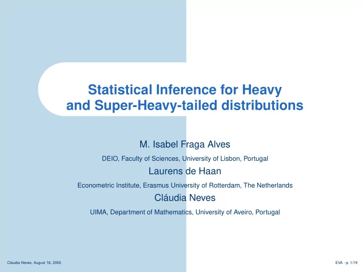
50 100 150 200 250 300 k
0.0 0.2 0.4 0.6 0.8
Beta=0.2 Beta=0.5 Std.LogPareto
LogWeibull and standard LogPareto
Mean
Patterns of the estimated mean of ˆ αn(k) log-Weibull distribution: F(x) = 1 − exp{−(log x)β}, x ≥ 1, 0 < β < 1 Standard log-Pareto distribution: FX(x) = 1 − (log x)−1, x ≥ e
50 100 150 200 250 300 k 0.0 0.2 0.4 0.6 0.8
Beta=0.2 Beta=0.5 Std.LogPareto
LogWeibull and standard LogPareto
Mean
Patterns of the estimated mean of the Hill estimator