
SLIDE 1
Different Payoffs Discontinuous Payoffs
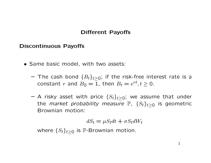
- Same basic model, with two assets:
Example: a digital option; for a digital call with strike K , 1 - - PowerPoint PPT Presentation
Different Payoffs Discontinuous Payoffs Same basic model, with two assets: The cash bond { B t } t 0 ; if the risk-free interest rate is a constant r and B 0 = 1, then B t = e rt , t 0. A risky asset with price { S t } t 0 ;