Evolution of the rate of evolution An analytical solution to the - PowerPoint PPT Presentation

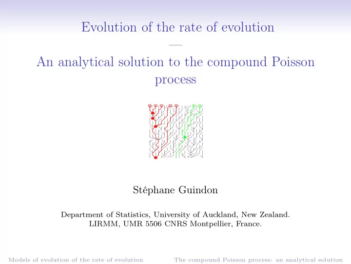
Evolution of the rate of evolution — An analytical solution to the compound Poisson process �� �� �� �� �� �� �� �� �� �� �� �� �� �� �� �� �� �� �� �� �� �� �� �� �� �� �� �� �� �� �� �� �� �� �� �� �� �� �� �� Stéphane Guindon Department of Statistics, University of Auckland, New Zealand. LIRMM, UMR 5506 CNRS Montpellier, France. Models of evolution of the rate of evolution The compound Poisson process: an analytical solution

Outline Models of evolution of the rate of evolution The compound Poisson process: an analytical solution Models of evolution of the rate of evolution The compound Poisson process: an analytical solution

A bit of history... • Linus Pauling and Emile Zuckerkandl (1962): “ molecular clock hypothesis ”. • Allan Wilson (1967): molecular dating under the molecular clock assumption. • 30 years passed... • Michael Sanderson (1997) and Jeffrey Thorne (1998): estimation of evolutionary divergence times without the restriction of a uniform rate across lineages. Models of evolution of the rate of evolution The compound Poisson process: an analytical solution

Molecular clock rate and time estimation ? t 2 ��� ��� ��� ��� ��������� ��������� � ��� ��� ��� ��� ��� ��� l 1 ��� ��� l 2 ��� ��� ��� ��� t 1 ������� ������� ��� ��� ��� ��� ��� ��� l 3 l 1 t 0 ��� ��� ��� ��� ��� ��� ������������ ������������ ��� ��� l 6 ������������ ������������ ��� ��� ��� ��� ��� ��� l 2 ��� ��� ��� ��� ��� ��� µ 1 ��� ��� ��� ��� ��� ��� l 5 ��� ��� ��� ��� ��� ��� l 5 l 4 � � ��� ��� ��� ��� t 1 ��� ��� ��� ��� ��� ��� ������������ ������������ � � ��� ��� ��� ��� ��� ��� ��� ��� ��� ��� ������������ ������������ ��� ��� l 6 ��� ��� ��� ��� ��� ��� ��� ��� ��� ��� ��� ��� ��� ��� ��� ��� ��� ��� µ 2 � l 4 ��� ��� ��� ��� ��� ��� ��� ��� ��� ��� l 3 ��� ��� ��� ��� ��� ��� l 7 l 7 ��� ��� ��� ��� l 8 ��� ��� ��� ��� ��� ��� ��� ��� ��� ��� ��� ��� ��� ��� l 8 t 0 ������������� ������������� ��� ��� ��� ��� t 2 ��� ��� ����� ����� ��� ��� ��� ��� ������������� ������������� ��� ��� ��� ��� ��� ��� ����� ����� l 4 + l 3 − l 1 − l 2 l 5 = µ × ( t 1 − t 0 ) µ 1 = t 0 − t 1 l 5 ֒ → µ = l 5 + l 6 + l 7 + l 8 − l 4 t 1 − t 0 µ 2 = t 1 − t 2 t 2 = l 1 + l 2 + l 3 + t 0 µ Models of evolution of the rate of evolution The compound Poisson process: an analytical solution

Beyond the molecular clock • Local clocks • Substitution rate is organised into a small number of classes, • Assign each branch to one of these classes. • Penalized likelihood • Ψ( R, T ) : penalty term for rate changes, • Maximise log ( P ( D | R, T )) − λ Ψ( R, T ) . • Bayesian approaches • Explicit stochastic models of the evolution of the substitution rate. • Rate trajectory is continuous or discrete. Models of evolution of the rate of evolution The compound Poisson process: an analytical solution

Models of rate evolution (1/2) • Log-normal model • µ is the mean of the rate at the nodes that begin and end the branch ( r (0) and r ( T ) ). • log ( r ( T )) ∼ N ( log ( r (0)) , νT ) . • Logarithm of the rate undergoes Brownian motion . • Correlation of mean rates on adjacent branches. • Exponential model • µ ∼ Exp ( φ ) . • No correlation of mean rates. • Shape of the distribution does not depend on time duration. Models of evolution of the rate of evolution The compound Poisson process: an analytical solution

Models of rate evolution (2/2) t 0 t 1 t 2 0 T r 0 r 1 r 2 r 3 • Compound Poisson process • Rates change in discrete jumps. • r ( t ) ∼ Γ( α, β ) • Number of jumps: n ( T ) ∼ Poisson ( λT ) • Correlation of mean rates across branches: governed by λ . • λT large: distribution of mean rate is approximately Normal. Models of evolution of the rate of evolution The compound Poisson process: an analytical solution

Implementation of the compound Poisson process • “Jump” event: Poisson ( λ ∆ t ) • Substitution rates: Γ( α, β ) t 0 t 0 t 0 r 0 r 0 r 2 t 1 t 1 r 1 t 1 r 2 r 2 • MCMC → posterior distribution of λ and α 1.0 0.6 0.8 Density Density 0.6 0.4 0.4 0.2 0.2 0.0 0.0 0 1 2 3 4 0.0 0.5 1.0 1.5 2.0 2.5 3.0 α λ Models of evolution of the rate of evolution The compound Poisson process: an analytical solution

Advantages and drawbacks • Log-normal • Computationally tractable • Crude (deterministic) description of the mean rates. • Biologically relevant ? • Exponential • Computationally tractable. • Distribution of mean substitution rate does not depend on time duration. • No correlation of mean rates across branches. • Compound Poisson • Description of rate changes plausible from a biological perspective. • Elegant way to account for correlation of mean rates across branches. • No analytical solution. Models of evolution of the rate of evolution The compound Poisson process: an analytical solution

Outline Models of evolution of the rate of evolution The compound Poisson process: an analytical solution Models of evolution of the rate of evolution The compound Poisson process: an analytical solution

First question t 0 t 1 t 2 0 T r 0 r 1 r 2 r 3 • r i ∼ Γ( α, β ) . Hence, E ( r i ) = αβ , V ( r i ) = αβ 2 . • n ∼ Poisson ( λT ) . • µ = � n i =0 k i r i , where k i = ∆ t i T . What is the distribution of µ ? • Work out the distribution of µ for a given value of n . • µ = � n i =0 k i r i is well approximated by a Gamma distribution. Models of evolution of the rate of evolution The compound Poisson process: an analytical solution

One jump t 0 0 T r 0 r 1 • µ = k 0 r 0 + (1 − k 0 ) r 1 • Distribution of t 0 = k 0 T ? λe − λx × e − λ ( T − x ) P ( t 0 = x | n = 1) = λTe − λT 1 = T . • k 0 ∼ U [0 , 1] → E ( k 0 ) = 1 1 2 and V ( k 0 ) = 12 . • E ( µ ) = E ( k 0 ) E ( r 0 ) + E (1 − k 0 ) E ( r 1 ) = αβ . • V ( µ ) = V ( k 0 r 0 ) + V ((1 − k 0 ) r 1 ) + 2 Cov ( k 0 r 0 , (1 − k 0 ) r 1 ) = 2 3 αβ 2 . Models of evolution of the rate of evolution The compound Poisson process: an analytical solution

n ≥ 1 jumps t 0 t 2 t 1 0 T r 0 r 1 r 2 r 3 • Distribution of k 0 ? λe − λx × ( λ ( T − x )) y − 1 e − λ ( T − x ) P ( t 0 = x | n = y ) = ( λT ) y e − λT /y ! y T y ( T − x ) y − 1 . = • After little algebra... 1 • E ( k 0 ) = n +1 , 2 • E ( k 2 0 ) = ( n +1)( n +2) . Models of evolution of the rate of evolution The compound Poisson process: an analytical solution

n ≥ 1 jumps t 0 t 2 t 1 0 T r 0 r 1 r 2 r 3 • µ = k 0 r 0 + k 1 r 1 + k 2 r 2 + k 3 r 3 . • µ n = k 0 r 0 + (1 − k 0 ) µ n − 1 . • E ( µ n ) = E ( k 0 ) E ( r 0 ) + E (1 − k 0 ) E ( µ n − 1 ) → E ( µ n ) = αβ . Models of evolution of the rate of evolution The compound Poisson process: an analytical solution

n ≥ 1 jumps t 0 t 1 t 2 0 T r 0 r 1 r 2 r 3 • The variance is a bit more challenging but can be done. V ( µ n ) = 2 αβ 2 + n ( n + 1) V ( µ n − 1 ) ( n + 1)( n + 2) • Solve the recursion: 2 n + 2 αβ 2 V ( µ n ) = Models of evolution of the rate of evolution The compound Poisson process: an analytical solution

Likelihood calculation • Data: • l , an expected number of substitutions. • T , elapsed time. • µ = l/T • Likelihood: ∞ � p µ ( u | λ, α, β, T ) = P ( n | λ, T ) p µ n ( u | α, β, n ) n =0 • P ( n | λ, T ) : Poisson distribution with mean and variance λT . • p µ n ( u | α, β, n ) : Gamma distribution with mean αβ , and 2 n +2 αβ 2 . variance Models of evolution of the rate of evolution The compound Poisson process: an analytical solution