estimation of local permeability with artificial
play

ESTIMATION OF LOCAL PERMEABILITY WITH ARTIFICIAL VISION TECHNIQUES - PDF document

18 TH INTERNATIONAL CONFERENCE ON COMPOSITE MATERIALS ESTIMATION OF LOCAL PERMEABILITY WITH ARTIFICIAL VISION TECHNIQUES USING A DIRECT METHOD L. Domnech 1 *, N. Monts 1 , F. Snchez 1 1 University of Cardenal Herrera, 46115 Alfara del


  1. 18 TH INTERNATIONAL CONFERENCE ON COMPOSITE MATERIALS ESTIMATION OF LOCAL PERMEABILITY WITH ARTIFICIAL VISION TECHNIQUES USING A DIRECT METHOD L. Doménech 1 *, N. Montés 1 , F. Sánchez 1 1 University of Cardenal Herrera, 46115 Alfara del Patriarca, Valencia (Spain) * Corresponding author ( luis.domenech@uch.ceu.es ) Keywords Numeric Analysis, LCM, Permeability, Artificial Vision 1. Introduction camera it is possible to define the pixels as nodes Measurement and characterization of fiber preform and associate them as Finite Elements. This fact permeability is one of the main issues in composites allows one using all the FE tools with the mesh process, since it plays a key role in process design defined by the camera. With this, mixed numerical/ and control. In fact, simulation is the only tool that experimental technique (MNET) is proposed to the allows guaranteeing a correct design and the success computation of the discretized space observed by the of the process, and the permeability is one critical camera as FE domain using a fixed mesh . With the input parameter needed by simulation. That’s the camera, it is possible to measure the arrival time at reason why in industry, it is needed that the which the flow achieves each node. Moreover, it is simulation and the reality are as close as possible, possible to measure the updating of the volume and so, the permeability must be as precise as fraction of each element and also the flow front possible. velocity since an amount of pixels can be associated However, in practice, permeability measurement is with each mesh. It permits to calculate the not a trivial task. In the literature of fibrous media percentage at which the mesh is filled. The pressure permeability [5][6][7][8], large variations in of each node cannot be measured but can be permeability values have been reported even in well- computed, given our possibilities to develop our controlled 1D or 2D flow experiments. It is found MNET. As the measurements are “directly” the that the permeability can vary largely from case to 
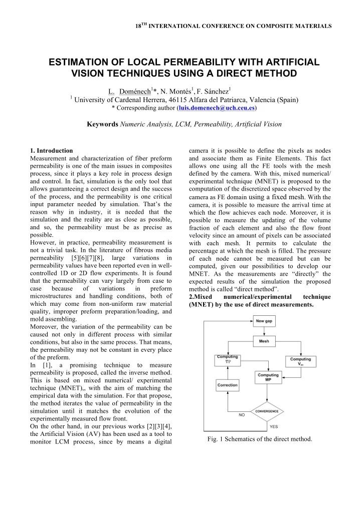
expected results of the simulation the proposed case because of variations in preform method is called “direct method”. microstructures and handling conditions, both of 2.Mixed numerical/experimental technique which may come from non-uniform raw material (MNET) by the use of direct measurements. quality, improper preform preparation/loading, and mold assembling. Moreover, the variation of the permeability can be caused not only in different process with similar conditions, but also in the same process. That means, the permeability may not be constant in every place of the preform. In [1], a promising technique to measure permeability is proposed, called the inverse method. This is based on mixed numerical/ experimental technique (MNET),, with the aim of matching the empirical data with the simulation. For that propose, the method iterates the value of permeability in the simulation until it matches the evolution of the experimentally measured flow front. On the other hand, in our previous works [2][3][4], the Artificial Vision (AV) has been used as a tool to Fig. 1 Schematics of the direct method. monitor LCM process, since by means a digital

  2. ! K + 1 " ! For one hand, the pressure in each node only can be ! r r obtained by FEM simulation. For the other hand it is V K ! K (1) possible to select the measured variables to work, as t K + 1 " t K well as the type of mesh, fixed mesh, moving mesh, ! K " ! etc If the updating of the volume fraction of each ! r r element is used to compute the material properties, V K ! K " 1 (2) t K " t K " 1 the goal of this equations is to obtain the velocity to compute the material properties by the Darcy´s law. ! K + 1 " ! The same occurs by the arrival time. For this ! r r K " 1 V K ! (3) reasons, the velocity computed by the camera is used t K + 1 " t K " 1 in our proposed method. Then, our MNET works as Where ! follows: for one hand, computed velocity by the K is the position of the pixel in the current r camera and the pressure obtained by the FEM flow front, ! K + 1 is the position of the closest pixel in r simulation is combined in the darcy´s law to obtain the next flow front and ! the material properties, see Fig.1 K ! 1 is the position of the r closest pixel in the previous flow front. 2.1 Meshing For the computation of the velocities of each FE, the For all the mesh possibilities that camera vision arithmetic mean of the velocities of the flow front allows, fixed mesh, moving mesh, etc, we choose a pixels which belong to each FE meshing procedure by means of the concatenation of triangularly meshed gaps defined by consecutive flow fronts, so that all the nodes belong to some flow front Fig. 2 Fig. 3 Pixels’ Velocities in the 5 th flow front. 2.3 FEM Numerical Velocity Computation Fig. 2 Meshing Procedure A previous work [9] shown how can be solved the That configuration allows guarantee that there are no numerical simulation of RTM mould filling. This partially filled elements and so, the nodes’ pressures method is used here in order to compute the pressure can be computed with higher accuracy. gradient in the fixed triangular mesh generated Moreover, with those characteristics, gradient through the artificial vision discretization. pressure is always perpendicular to the flow front so Darcy’s law can model the resin flow through a that, the velocity vector and gradient pressures are porous medium: collinear. ! V = ! K " # µ $ P (4) 2.2 Obtaining Velocity by means Artificial Vision Computation of velocities at flow front can be ! V is the velocity vector, ! is the porosity, µ where estimated by means the distance and time between is the viscosity, P is the pressure and K is a consecutive flow fronts. To compute pixels’ velocities a numerical approximation of velocity is permeability tensor. applied, concretely the forward(1), backward(2) and The fluid flow problem is defined in a volume Ω , central(3) difference method in the initial, final and intermediate flow fronts respectively. ( t )  ( t ) (5) Ω = Ω Ω f e

  3. ESTIMATION OF LOCAL PERMEABILITY WITH ARTIFICIAL VISION TECHNIQUES USING A DIRECT METHOD In our proposal, the meshing algorithm is developed where the fluid at time t occupies the volume Ω f (t) in order to include all the control volumes that are and Ω e (t) defines at that time the empty part of the completely filled, so that I=1. That information is mold. Assuming fluid incompressibility, the obtained directly from the artificial vision as stated variational formulation related to the Darcy flow before. So in the method proposed, the updating of results the volume fraction is not calculated with Eq.(8). $ ' K This equation, and hence step 3, is only used in + ! p * " # " µ ! p d * = 0 & ) (6) terms on the numerical evaluation of the proposed % ( ( ) * f t method. where p* denotes the usual weighting function. The prescribed conditions to impose on the boundary of Ω f (t) are: • The pressure gradient in the normal direction to the mold walls is zero. • The pressure or the flow rate is specified at the injection nozzle. • Zero pressure is applied on the flow front. The flow kinematics can be computed by means of a conforming finite element Galerkin technique Fig. 4 Fixed triangular mesh with control volumes in applied to the variational formulation extended to elements and computation of numerical flow the whole domain Ω velocities in elements 3. Estimation of Material Properties The location of the fluid into the whole domain Ω is defined by the characteristic function I defined by In this section a methodology for estimating the local Material Properties based on Artificial Vision 1 x ( ) t ∈ Ω ⎧ is described. ⎪ f I ( x , t ) (7) = ⎨ ( ) 0 x t As has been shown in (4) Darcy’s law describes the ∉ Ω ⎪ ⎩ f behavior of fluid in a porous medium. The evolution of the volume fraction, I , is given However, if the porous medium is isotropic, tensor by the general linear advection equation: K can be replaced by a number since K xx = K xy = K so that, equation (4) can be dI I ∂ v I 0 (8) = + ⋅ ∇ = expressed as (9), dt t ∂ with I=1 on the inflow boundary. V = M ! " P (9) So that, the resolution scheme is based in solving the three steps: Where M = K represents the Material Properties 1. Obtain the pressure field using a finite ! ! µ elements discretization of the variational (MP), and the tensorial dimension has been removed formulation given by Eq. (6) and imposing since both vectors are collinear. null pressure in the nodes contained by an So that M can be computed as follows empty element (i.e nodes 4, 5 and 6 in Fig. 4 ). M = V AV 2. Compute the pressure gradient and the (10) ! P velocity field from Darcy´s law 3. Update the element volume fraction, I, integrating the equation (8) 3

Download Presentation
Download Policy: The content available on the website is offered to you 'AS IS' for your personal information and use only. It cannot be commercialized, licensed, or distributed on other websites without prior consent from the author. To download a presentation, simply click this link. If you encounter any difficulties during the download process, it's possible that the publisher has removed the file from their server.

Recommend


More recommend