Enhancing Prediction Accuracy In Sift Theory J. Wang 1 *, W. K. Chiu - - PDF document

SLIDE 1

18TH INTERNATIONAL CONFERENCE ON COMPOSITE MATERIALS

1 Introduction In the conventional laminate theory widely used to predict the strength of fibre-reinforced polymer composites, the laminae are treated as homogeneous

• rthotropic materials. Gosse and Christensen [1]

adopted a micromechanical approach which predicts separately the failure of the polymer matrix and

• fibres1. They used strain invariants as failure criteria

and thus this approach was named as Strain Invariant Failure Theory (SIFT). In the application of SIFT, a microstructure analysis is conducted on a unit cell of the composite material that contains a fibre and surrounding polymeric matrix to determine the relationship between the stress-strain states of the whole cell and its matrix and fibre

• components. This relationship is then used in a

structural analysis to predict matrix or fibre failure. In a linear finite element method, the SIFT analysis could be implemented during post processing the results from a computation based on the conventional laminate theory, by correlating the element stress- strain state with matrix and fibre stress-strain states. This theory has been used by a number of researchers and some success has been reported [2]. For the matrix failure prediction, Gosse and Christensen proposed that two properties that control damage in the matrix, are the first invariant of the strain tensor,

,

1ε

J

and the second invariant deviator,

eqv

ε

:

3 2 1 1

ε ε ε + + =

ε

J

(1)

{

}

5 . 2 3 2 2 3 1 2 2 1

] ) ( ) ( ) [( 5 . ε ε ε ε ε ε ε − + − + − =

eqv

(2) where

3 2 1

, , ε ε ε

are principal strains.

1 In principle this micromechanical approach may also

predict the interfacial failure between the fibre and matrix.

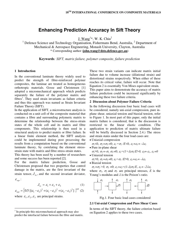
These two strain variants can indicate matrix initial failure due to volume increase (dilational strain) and distortional strains respectively. When either of these reaches its critical value, failure will occur. Note that Equation 2 is essentially Von Mises equivalent strain. This paper aims to demonstrate the accuracy of matrix failure prediction could be increased significantly by enhancing these two failure criteria. 2 Discussion about Polymer Failure Criteria In the following discussion four basic load cases will be considered, namely uni-axial compression, pure in- plane shear, uniaxial tension and biaxial tension, refer to Figure 1. In most part of this paper, only the initial matrix failure is considered, that is the discussion is restricted to the linear elastic condition. (The application to prediction of matrix ultimate failure will be briefly discussed in Section 2.4.) The stress and strain states under the four load cases are:

• Uniaxial compression

σ1<0, σ2 =σ3 =0; ε1 =σ1 /E<0, ε2 =ε3 = -λε1

• Pure in-plane shear

σ1>0, σ2 =-σ1, σ3 =0; ε1=(1+λ)σ1/E>0, ε2=-ε1, ε3 =0

• Uniaxial tension

σ1>0, σ2 =σ3 =0; ε1=σ1 /E>0, ε2 =ε3 = -λε1

• Biaxial tension

σ1 =σ2 >0, σ3 =0; ε1 =ε2=(1-λ)σ1/E, ε3 = -2λε1 where σ1, σ2 and σ3 are principal stresses, E is the Young’s modulus and λ is the Poison’s ratio. Fig.1. Four basic load cases considered 2.1 Uni-axial Compression and Pure Shear Cases In terms of the SIFT theory, the failure criterion based

• n Equation 2 applies to these two cases.

Enhancing Prediction Accuracy In Sift Theory

• J. Wang1*, W. K. Chiu2

1 Defence Science and Technology Organisation, Fishermans Bend, Australia, 2 Department of

Mechanical & Aerospace Engineering, Monash University, Clayton, Australia

* Corresponding author (john.wang@dsto.defence.gov.au)

Keywords: SIFT, matrix failure, polymer composite, failure prediction

σ1 σ1 σ1 σ1 σ2 σ2

SLIDE 2

2

It is well known that the strength of polymer materials could be affected by compressive hydrostatic stress. For those polymer materials, to cover both uniaxial compression and pure shear load cases, a yield criterion such as the Drucker-Prager criterion 2 [3] would be more suitable than Von Mises criterion. Table 1 provides yield strength data for two typical resin materials used in laminate composites. Table 1. Typical resin material strength data [4]

Resin Tensile (MPa) Compression (MPa) Shear (MPa) Yield strength 58 96 50 Type 1 E=3.6GPa λ=0.35 Ultimate strength 58 130 62 Yield Strength 50 100 36 Type 2 E=3.9GPa λ=0.35 Ultimate strength 50 130 60

For the prediction of yield strength, if we generate the critical value of

eqv

ε

from pure shear data, the measured yield strength in the uni-axial compression case will be higher than the predicted using Equation 2 by 11% and 60% respectively for these two

• materials. This discrepancy can be removed by

applying the 2-parameter Drucker-Prager criterion (based on Equation 3).

A BJ

eqv

= +

ε

ε

1

(3) where

eqv

ε

and

1

J are calculated using Equations 1

and 2 with the measured failure data from compression and shear tests (Table 1); A and B are two parameters determined from this equation. Failure is predicted when:

A BJ

eqv eqv

= + =

ε

ε ε

1

'

(4) where

eqv

' ε

is the revised equivalent strain. Equations (5) and (6) below describe the first invariant of the stress tensor,

,

1σ

J

and the second stress invariant deviator,

eqv

σ

:

3 2 1 1

σ σ σ

σ

+ + = J

(5)

{

}

5 . 2 3 2 2 3 1 2 2 1

] ) ( ) ( ) [( 5 . σ σ σ σ σ σ σ − + − + − =

eqv

(6)

2 Only basic failure criteria that are relatively easy to

implement are considered in this study.

Note the following relationship:

E

eqv eqv

λ σ ε + = 1

(7)

E J J λ

σ ε

2 1

1 1

− =

(8) The failure prediction equations can alternatively be expressed using stress variables with full equivalence. For isotropic materials, a stress based failure criterion is more commonly used since it is often easier to use and have clearer physical meaning (e.g. hydrostatic pressure effect shown in Drucker-Prager criterion). Alternative equations of Equations (3) and (4) expressed in stresses are:

A BJ

eqv

= +

σ

σ

1

(9)

A BJ

eqv eqv

= + =

σ

σ σ

1

'

(10) For the materials listed in Table 1, A and B values calculated are listed in Table 2. Table 2. Parameter A and B values

Strain based equation Stress based equation Resin A B A B Type 1 32.5x103µε 0.439 86.6MPa 0.098 Type 2 21.6x103µε 1.69 62.4MPa 0.376

2.2 Uni-axial and Biaxial Tension Cases Before discussing the uni-axial and biaxial tension cases, we may consider an extreme case where the polymer is loaded with uniformly distributed tensile stress in all the three axial directions. It is well known that the Von Mises yield criterion is not valid in this

• situation. A Drucker-Prager criterion established using

parameters determined from compression and shear load cases would also significantly over-predict the strength in this situation. One commonly adopted approach is to use a maximum tensile stress or strain criterion to handle such tensile dominated load conditions, in conjunction with other criteria such as Von Mises or Drucker-Prager to handle other load

• conditions. In contrast, Equation 1 adopted by Gosse

and Christensen contains all the 3 principal strain components in linear combination that indicates the volume increase of the material. Bardenheier [5-6] provided experimental data from uni-axial and biaxial tension tests of three types of polymer materials. Analysing these data, it is indicated that under a biaxial tensile load condition, prediction based on Equation 1 would significantly

SLIDE 3

3

J1σUT J1σ’UT σeqvUC

σeqv’ST σeqv’CS

σ1 σ2 under-estimate the material strength, refer to Table 3. The dilational failure could be more accurately predicted using the critical value of, for example:

5 . 2 3 2 2 2 1 1

) ( ' σ σ σ

σ

+ + = J

(11) This fits more closely to the experimental results. Note that as principal stresses are used, Equation 11 is unaffected by any transformation of coordinates. Table 3. Data from neat resin biaxial tests [5-6] and errors with different prediction methods

Stress applied* Error with prediction method** (%) Resin σ1 σ2 Eqn (1) Eqn (11) Max stress criterion Type A 0.79 0.79

• 36.7
• 10.5

+21.0 Type B 0.84 0.50

• 25.4

+2.3 +16.0 Type C 0.85 0.80

• 39.4
• 14.3

+15.0 * Expressed using the ratio of the yield stress in the biaxial test against that in the uni-axial tensile test ** In each method, the yield stress from the uni-axial tensile test was used to determine the critical value for prediction of yield strength in biaxial tests. A “+” sign means over-prediction and a “-“ sign means under- prediction.

2.3 Combined Failure Envelope Figure 2 illustrates a failure envelope with the plane- stress condition (σ3 ≡ 0). The portion of the failure envelope formed with the Drucker-Prager failure criterion has two parts. The solid line part (σeqv’CS) is established with the uni-axial compression and pure shear test data as discussed in Section 2.1, whilst the fine dot line part (σeqv’ST) is established with the pure shear and uni-axial tensile data in a similar way. This figure shows that the portion of the failure envelope formed with the Drucker-Prager failure criterion can intersect with uni-axial compression, pure shear and uni-axial tensile test data points and join with the J1σ’ curve smoothly, that indicates significantly improvement. (Regarding the curve smoothness, note that a significant improvement of the Von-Mises criterion over the maximum shear (Tresca) criterion is that it smooths the curve and removes the singular points in Tresca criterion.) In the 3-dimensional space with σ1, σ2, σ3 coordinate axes, the failure envelope is represented by two cone surfaces (formed with the Drucker-Prager failure criterion, with the axis along the line σ1 = σ2 = σ3 and joined at σ1 +σ2 +σ3 = 0) truncated by a hemisphere surface (formed with J1σ’ = the uni-axial tensile yield stress).

UT = uni-axial tensile; BT = biaxial tensile; PS = pure shear; UC = uni-axial compression; σeqvUC = σeqv with critical value determined from uni-axial compression test; σeqv’CS = σeqv’ with parameters determined from uni-axial compression and shear tests; σeqv’ST = σeqv’ with parameters determined from shear and uni-axial tensile tests; J1σUT = J1σ with critical value determined from uni-axial tensile test; and J1σ’UT = J1σ’ with critical value determined from uni-axial tensile test.

Fig.2. Illustration of failure envelope (plane-stress) 2.4 Matrix Ultimate Failure Prediction By using the ultimate strength and secant stiffness to replace yield strength and initial linear stiffness, the above analysis may be extended to cover prediction of matrix ultimate failure with linear analyses. Note that:

• The accuracy of Drucker-Prager criterion over Von

Mises failure criterion has been clearly observed particularly for the ultimate strength of many polymer materials; and

• Use of a linear analysis with secant stiffness to

approximate a nonlinear analysis is a widely used analysis method and thus may be significant for practical applications. 3 Lamina Unit Cell Analysis A unit cell analysis using a finite element method was further conducted with the four typical load cases discussed above. The failure prediction based on Equation (1) and Equation (2) was compared with that based on Equations (10) and (11) when both fibre and matrix are present.

SLIDE 4

4

As the discussion in Section 2 indicated that the failure criteria proposed in this paper could predict neat resin failure more accurately, Equations (10) and (11) are used as a yardstick in this comparison. 3.1 Finite Element Model The following typical material properties are assumed:

• Fibre Young’s modulus (Ef)

= 200 GPa

• Fibre Poisson ratio (λf)

= 0.3

• Matrix Young’s modulus (Em)

= 3.6 GPa

• Matrix Poisson ratio (λm)

= 0.35

• Fibre volume fraction (Vf)

= 0.5 Referring to Figure 3, with a relatively low fibre volume fraction of 0.5, a “square” pattern fibre distribution in the matrix can be assumed (as opposed to a “hexagon” pattern). A unit cell was extracted with two different orientations. A FEM model is shown in Figure 4. Considering the symmetrical condition, only

• ne eighth of the unit cell was built.

(a) Orientation 1 (b) Orientation 2 Fig.3. Unit cells with two orientations (Vf = 0.5) Fig.4. A unit cell FEM mesh (one-eighth model of the unit cell in Figure 3a) The load condition is applied in the form of uniform surface displacement. Symmetry boundary conditions are applied to three orthogonal surfaces. The remaining unloaded surfaces were given a uniform displacement, that results in the gross load on the surface being zero, to reflect the “Poisson effect”. The loading and boundary conditions applied ensure all the surfaces are kept straight, as required for simulation of a unit cell in a lamina structure. 3.2 Results and Discussion 3.2.1 Compression and Shear Load Cases The unit cell shown in Figure 3(a) was considered. As expected, for the matrix material in the uni-axial compression case, high compressive stress concentration (over 4 times the average strain of the unit cell) occurred at the area indicated in Figure 5(a). Due to the Poisson effect from the stiff fibre, the other two stress components perpendicular to the applied load are also compressive in the high stress concentration area. This results in a relatively high hydrostatic stress in this area and thus the strength predicted with the Drucker-Prager type criterion is much higher than that with Von-Mises criterion. In contrast, in the pure-shear case, high compressive and tensile stress concentration occurred separately at the areas shown in Figure 5(b). This results in strength predicted with Drucker-Prager type criterion to be much less than that with Von-Mises criterion in the tensile stress concentration area. (a) (b) Fig.5. Stress concentration areas in uni-axial compression and “pure shear” load cases With a load applied that resulted in 0.01 gross strain, the calculated maximum effective stress values are listed in Table 4. For practical applications of the SIFT approach, the failure strength of the matrix is generally determined using laminate specimen tests rather than from neat

Compression stress concentration area Tensile stress concentration area

SLIDE 5

5 b a a b a a

resin tests3 [1]. If the strength is calibrated using the uni-axial compression strength for Material Type 1 (Table 1), when predicting strength in the pure-shear load case, as indicated in Table 4, the difference between the original SIFT approach and the proposed revised approach is 60.6%. Table 4. Predicted maximum εeqv and σeqv’ values under uni-axial compression and pure-shear loadings

(1) Uni-axial compression (2) Pure- shear Ratio (2)/(1) Discrepancy εeqv 0.0574 0.0624 1.09 σeqv’ 1.14E2 MPa 2.00E2 MPa 1.75 60.6%

3.2.2 Uni-axial and Biaxial Tension Load Cases Figure 6 shows the stress concentration areas in these two load cases for the unit cell shown in Figure 3(a). In the biaxial tension case, each of the two stress concentration areas was affected mainly by one of the two loads. Thus there is no significant biaxial tensile

• stress. Table 5 lists maximum J1ε and J1σ‘ values.

Consequently when using the two different methods calibrated using uni-axial tensile state data to predict biaxial state strength, the difference is only 3.4%. (a) (b) Fig.6. Stress concentration areas in uni-axial and biaxial tension load cases - Orientation 1. The unit cell shown in Figure 3(b) was subsequently

• calculated. The maximum critical value locations in

the uni-axial tensile load case are at “a” positions shown in Figure 7 (a), whilst the maximum critical

3 The effect of scale difference between the unit cell and

lamina structure is generally not considered in SIFT, refer to [1], whilst this calibration may, to certain degree, take the scale effect into consideration.

value locations in the biaxial tensile load case are at “b” positions shown in Figure 7(b). These maximum critical values listed in Table 6. Table 5. Predicted maximum J1ε and J1σ’ values under uni-axial and biaxial tension loadings - Orientation 1

(1) Uni-axial tension (2) Biaxial tension Ratio (2)/(1) Discrepancy J1ε 0.0376 0.0438 1.18 J1σ’ 2.73E2 MPa 3.12E2 MPa 1.14 3.4 %

(a) (b) Fig.7. Stress concentration areas in uni-axial and biaxial tension load cases - Orientation 2. As shown in Table 6, when using the two different methods calibrated using uni-axial tensile state data to predict biaxial state strength, the difference is 6.1%, in terms of the maximum critical values in the whole matrix, however, for a specific critical location such as at “b” locations, the two methods yield significant

• difference. This might have a complicated effect on

determining the correlation between the element stress-strain and matrix and fibre stress-strain states. Table 6. Predicted J1ε and J1σ’ values at critical points under uni-axial and biaxial tension loadings - Orientation 2

(1) Uni-axial tension (2) Biaxial tension Ratio (2)/(1) Difference J1ε 0.0141 0.0334 2.37 Point a J1σ’ 1.05E2 MPa 2.44E2 MPa 2.32 1.0 % J1ε 0.00978 0.0435 4.44 Point b J1σ’ 1.02E2 MPa 3.05E2 MPa 2.98 49.0 % J1ε 0.0141 0.0435 3.09 Max J1σ’ 1.05E2 MPa 3.05E2 MPa 2.90 6.1 % Tensile stress concentration areas

SLIDE 6

6

4 Summary

• The SIFT failure theory separably predicts fibre

and matrix failure in a fibre reinforced composite

• material. Matrix yield prediction is based on a

Von-Mises strain and first strain invariant criteria. Improvement of the matrix failure criteria for prediction accuracy is discussed and demonstrated in this paper.

• For two typical resin materials, Von-Mises yield

criterion is unable to fit both yield strength values from uni-axial compression and pure-shear tests. When calibrated using the measured shear yield strength, the discrepancy between the predicted and measured uni-axial compression strength is found to be 11% and 60% respectively, whilst using a Drucker-Prager criterion these discrepancies could be removed.

• Use of the critical value of the first invariant

strain, when calibrated using the uni-axial tensile yield strength, under-predicts the biaxial tensile strength significantly by over 30% on average, compared with available measurement data of neat resin materials. A revised criterion proposed in this paper could reduce the discrepancy to less than 10%.

• The proposed failure envelope contains Drucker-

Prager failure criteria, that intersect with all the uni-axial compression, pure shear and uni-axial tensile test data points, and a revised tensile failure criterion. The areas governed by these criteria join each other smoothly.

• For a unit cell with a fibre and surrounding matrix

from a lamina with 50% fibre volume fraction and typical material properties, a FEM analysis conducted in this study indicates that the difference between the yield strength of the matrix material predicted using Von-Mises and Drucker- Prager type criteria is over 60% in the pure shear load case, when the critical values of these yield criteria are determined in the uni-axial compression load case.

• The FEM analysis showed that the difference

between the yield strength of the matrix material in a unit cell predicted using the first strain variant and the revised criterion reaches 6.1% in the biaxial tensile load case, when the critical values

• f these yield criteria are determined in the uni-

axial tensile load case.

• By using ultimate strengths and secant stiffness to

replace yield strengths and initial linear stiffness, the analysis in this paper may be extended to prediction of matrix ultimate failure using linear analyses. Acknowledgement The authors would like to acknowledge that this paper is outcome of a research project of the Cooperative Research Centre for Advanced Composite Structures (CRC-ACS). References

[1] Gosse JH, Christensen S., “Strain invariant failure

criteria for polymers in composite materials”, AIA

• A. Paper 2001-1184. AIAA/ASME/ASCE/ASC

conference, Seattle, WA, United States, 2001.

[2] Li R, Kelly D, and Ness R. Application of a first

invariant strain criterion for matrix failure in composite materials. Journal

• f

composite Materials, 2003. 37(22): 1977-2000.

[3] Drucker D C and Prager W. “Solid mechanics and

plastic analysis for limit design. Quarterly of Applied Mathematics, 10 (2). 157-165, 1952.

[4] Fei Y P. Mechanics of fibre reinforced composite.

Tongji University Press. Shanghai. 1981.

[5] Bardenheier. Mechanicaches Versagen von

• Polymerwerkstooen. Hanser-Verlag. 1982.

[6] Kolling S, Haufe A, Feucht M, and Du Bois P A.

A constitutive formulation for polymers subjected to high strain rates. 9th International LS-Dyna Users Conference. Michigan, June 4-6, 2006.