[PDF] - Einfhrung in Visual Computing Unit 5: Image Encoding and Compression PDF Document

SLIDE 1

12.03.2013 1

Einführung in Visual Computing

Unit 5: Image Encoding and Compression

Content:

http://www.caa.tuwien.ac.at/cvl/teaching/sommersemester/evc

Introduction to Encoding
Image File Formats
Information vs. Data
Introduction into

Compression

Lossless Compression
Lossy Compression
Video Compression

1 Robert Sablatnig, Computer Vision Lab, EVC‐5: Image Encoding and Compression

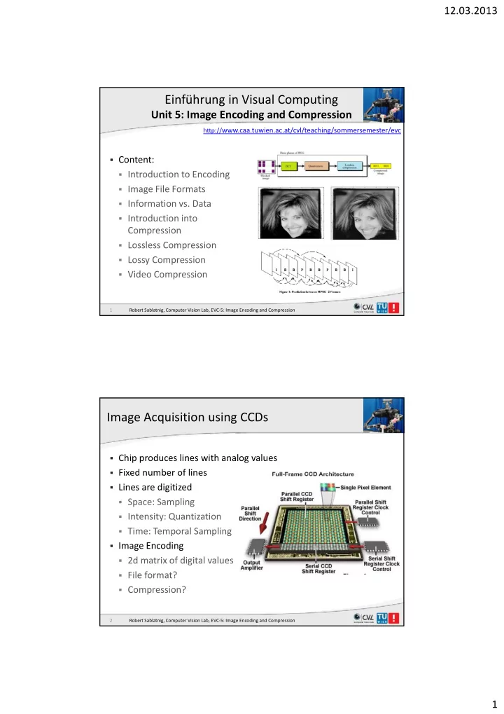
Image Acquisition using CCDs

Chip produces lines with analog values
Fixed number of lines
Fixed number of lines
Lines are digitized
Space: Sampling
Intensity: Quantization
Time: Temporal Sampling
Image Encoding

g g

2d matrix of digital values
File format?
Compression?

Robert Sablatnig, Computer Vision Lab, EVC‐5: Image Encoding and Compression 2

SLIDE 2

12.03.2013 2

3 Robert Sablatnig, Computer Vision Lab, EVC‐5: Image Encoding and Compression

Storage Requirements for Digital Images

Image LxN pixels, 2B gray levels, c color components
Example: L=N=512, B=8, c=1 (i.e., monochrome)

Size = 2,097,152 bits (or 256 kByte) , , ( y )

Example: LxN=1024x1280, B=8, c=3 (24 bit RGB image)

Size = 31,457,280 bits (or 3.75 MByte)

Much less with (lossy) compression!

4 Robert Sablatnig, Computer Vision Lab, EVC‐5: Image Encoding and Compression

SLIDE 3

12.03.2013 3

Image/Graphics Files

Images (Bit )

Text

2D Vector- hi 3D Vector- hi (Bitmaps)

Text

graphics graphics

5 Robert Sablatnig, Computer Vision Lab, EVC‐5: Image Encoding and Compression

What are the Categories?

One categorization:

Raster Image Formats
Raster Image Formats
Vector Image Formats

Another categorization:

Binary Image Formats
ASCII Image Formats

g

6 Robert Sablatnig, Computer Vision Lab, EVC‐5: Image Encoding and Compression

SLIDE 4

12.03.2013 4

Raster Image Formats

7

Raster Image Formats

Breaks the image into a series of color dots called “pixels”
The number of bits at each pixel determines the maximum number
The number of bits at each pixel determines the maximum number
f colors

1 bits = 2 (21) colors 2 bits = 4 (22) colors 4 bits = 16 (24) colors 8 bits = 256 (28) colors 16 bits = 65,536 (216) colors 24 bits = 16,777,216 (224) colors

Examples:
BMP/DIB: BitMaP or Device Independent Bitmap (DIB), Microsoft

Windows and OS/2

PBM, PGM, PPM: Portable BitMap, GrayMap, PixMap, Unix, PC
TGA: Truevision Advanced Raster Graphics Adapter (TARGA), Avi

8 Robert Sablatnig, Computer Vision Lab, EVC‐5: Image Encoding and Compression

SLIDE 5

12.03.2013 5

Example: BMP Format

The bitmap image file consists of:
fixed‐size structures (headers)
variable‐size structures (image)

Robert Sablatnig, Computer Vision Lab, EVC‐5: Image Encoding and Compression 9

Raster Image Formats

10 Robert Sablatnig, Computer Vision Lab, EVC‐5: Image Encoding and Compression

SLIDE 6

12.03.2013 6

Instead …

11 Robert Sablatnig, Computer Vision Lab, EVC‐5: Image Encoding and Compression

Vector Image Formats

12

SLIDE 7

12.03.2013 7

Vector Image Formats

Break the image into a set of mathematical descriptions
f shapes: curve arc rectangle sphere etc
f shapes: curve, arc, rectangle, sphere etc.
Resolution‐independent: scalable without the problem
f “pixelating”.
Not all images are easily described in a mathematical

form. H t d ib h t h?

How to describe a photograph?

13 Robert Sablatnig, Computer Vision Lab, EVC‐5: Image Encoding and Compression

Vector Image Formats

Break the image into a set of mathematical descriptions
f shapes: curve arc rectangle sphere etc
f shapes: curve, arc, rectangle, sphere etc.
Resolution‐independent: scalable without the problem
f “pixelating”.
Not all images are easily described in a mathematical

form. H t d ib h t h?

How to describe a photograph?

14 Robert Sablatnig, Computer Vision Lab, EVC‐5: Image Encoding and Compression

SLIDE 8

12.03.2013 8

CGM

Goal: to make vector graphics portable across different operating

systems

Computer Graphics Metafile: 3 types of coding
Raster / vector format, ANSI standard for exchange of image data

between different graphics software (device independent). Metafile contains data and information, which describes the organization and the semantics of the data. Due to the structuring of CGM is an ideal partner for HTML and SGML.

1999: "Application Structuring,“ enables to use non‐graphic

f ( information along with graphic content (interactive graphics, "Hot Spots,hyperlinks, etc.)

Different application profiles: define options, elements and

parameters necessary to enable specific functions and the interchangeability of the systems

15 Robert Sablatnig, Computer Vision Lab, EVC‐5: Image Encoding and Compression

WMF ‐ Windows MetaFile

Graphics file format on Microsoft Windows systems, originally

designed in the 1990s. Windows Metafiles are intended to be g portable between applications and may contain both vector graphics and bitmap components.

WMF file stores a list of function calls that have to be issued to

the Windows Graphics Device Interface (GDI) layer to display an image on screen.

EMF (Enhanced Metafile) 32bit extension to 16bit‐ WMF

EMF (Enhanced Metafile) 32bit extension to 16bit WMF

EMF+ with Windows XP

16 Robert Sablatnig, Computer Vision Lab, EVC‐5: Image Encoding and Compression

SLIDE 9

12.03.2013 9

Comparison

Raster

R l ti d d t

Vector

R l ti i d d t

‐ Resolution‐dependent ‐ Suitable for photographs ‐ Smooth tones and subtle

details

‐ Larger size ‐ Resolution‐independent ‐ Suitable for line drawings,

CAD, logos

‐ Smooth curves ‐ Smaller size

17 Robert Sablatnig, Computer Vision Lab, EVC‐5: Image Encoding and Compression

Image Compression

18

SLIDE 10

12.03.2013 10

Goal of Image Compression

Digital images require huge amounts of space for storage and

large bandwidths for transmission. g

A 640 x 480 color image requires close to 1MB of space.
The goal of image compression is to reduce the amount of data

required to represent a digital image.

Reduce storage requirements and increase transmission rates.

19 Robert Sablatnig, Computer Vision Lab, EVC‐5: Image Encoding and Compression

Data ≠ Informaon

Data and information are not synonymous terms!
Data is the means by which information is conveyed.
Data compression aims to reduce the amount of data required to

represent a given quantity of information while preserving as much information as possible.

20 Robert Sablatnig, Computer Vision Lab, EVC‐5: Image Encoding and Compression

SLIDE 11

12.03.2013 11

Data vs Information (cont’d)

The same amount of information can be represented by

i t f d t various amount of data, e.g.:

Your wife, Helen, will meet you at Logan Airport in Boston at 5 minutes past 6:00 pm tomorrow night Your wife will meet you at Logan Airport at 5 minutes past 6:00 pm tomorrow night

Ex1: Ex2:

Helen will meet you at Logan at 6:00 pm tomorrow night

Ex3:

21 Robert Sablatnig, Computer Vision Lab, EVC‐5: Image Encoding and Compression

Data Redundancy

compression Compression ratio:

22 Robert Sablatnig, Computer Vision Lab, EVC‐5: Image Encoding and Compression

SLIDE 12

12.03.2013 12

Data Compression

Data compression implies sending or storing a smaller number of

bits.

lossless and
lossy methods.
Trade‐off: image quality vs compression ratio

23 Robert Sablatnig, Computer Vision Lab, EVC‐5: Image Encoding and Compression

Lossless Image Compression

24

SLIDE 13

12.03.2013 13

Run Length Encoding (RLE)

Spatial and temporal neighboring pixels have similar intensity

(colors) ( )

spatial temporal

25 Robert Sablatnig, Computer Vision Lab, EVC‐5: Image Encoding and Compression

Run Length Encoding (RLE)

Simplest method of compression
Can be used to compress data made of any combination of
Can be used to compress data made of any combination of

symbols, does not need to know the frequency of occurrence of symbols

Replace consecutive repeating occurrences of a symbol by one
ccurrence of the symbol followed by the number of occurrences

Original

Lossless compression!

Robert Sablatnig, Computer Vision Lab, EVC‐5: Image Encoding and Compression 26

2 3 4 6 3 Original Coded

SLIDE 14

12.03.2013 14

Huffman Coding

Assigns shorter codes to symbols that occur more frequently and

longer codes to those that occur less frequently. g q y

Example text file with five characters (A, B, C, D, E):
Assign each character a weight based on its frequency of use

27 Robert Sablatnig, Computer Vision Lab, EVC‐5: Image Encoding and Compression

Huffman Encoding

28 Robert Sablatnig, Computer Vision Lab, EVC‐5: Image Encoding and Compression

SLIDE 15

12.03.2013 15

Huffman Encoding

Character code found by starting at the root and following the

branches that lead to that character.

The code itself is the bit value of each branch on the path, taken

in sequence.

Decoding: reverse process

Robert Sablatnig, Computer Vision Lab, EVC‐5: Image Encoding and Compression 29

Lempel Ziv (LZ) Dictionary‐based Encoding

Dictionary is a table of strings
Sender and receiver have a copy of dictionary
Previously encountered strings are substituted by their index in
Previously‐encountered strings are substituted by their index in

dictionary

Compression ‐ two concurrent events:
Building an indexed dictionary
Compressing a string of symbols.
Algorithm extracts smallest substring not in the dictionary from

remaining uncompressed string.

Stores a copy of this substring in dictionary as a new entry and assigns it

Stores a copy of this substring in dictionary as a new entry and assigns it an index value.

Compression occurs when substring (except for the last character) is

replaced with the index found in the dictionary.

Process inserts the index and the last character of the substring into the

compressed string.

30 Robert Sablatnig, Computer Vision Lab, EVC‐5: Image Encoding and Compression

SLIDE 16

12.03.2013 16

Example of Lempel Ziv Encoding

Robert Sablatnig, Computer Vision Lab, EVC‐5: Image Encoding and Compression 31

Lossless Image Formats

GIF‐Format (Graphics Interchange Format)
LZW‐Compression (Lempel, Ziv, Welch): works line‐wise
1 st line, 2nd line
3rd line is compressed as:
1 white, 1 yellow, 5 red, 2 yellow, 1 green
Row 4 to 6: „as row 3“
Indexed (1‐8 bit Color Lookup Table)

32 Robert Sablatnig, Computer Vision Lab, EVC‐5: Image Encoding and Compression

SLIDE 17

12.03.2013 17

CompuServ GIF (gif)

First standardized in 1987 by CompuServ (called GIF87a)
Updated in 1989 to include transparency interlacing and
Updated in 1989 to include transparency, interlacing, and

animation (called GIF89a)

Use the LZW (Lempel‐Ziv Welch) algorithm for compression (not

free, licenses necessary)

A maximum of 256 colors freely selectable out of 24 bit (224 =

16.777.216) D k f h h

Does not work for photographs
Suitable for small images such as icons
Simple animations

33 Robert Sablatnig, Computer Vision Lab, EVC‐5: Image Encoding and Compression

p ( )

Robert Sablatnig, Computer Vision Lab, EVC‐5: Image Encoding and Compression 34

SLIDE 18

12.03.2013 18

Tagged Image File Format (tiff)

originally created as an attempt to get desktop scanner vendors of

1985 to agree on a common scanned image file format, rather g g , than have each company promote its own proprietary format

Aldus/Microsoft/Adobe
Flexible and extendible because of „tags“
Indexed or True‐color
Compressed/uncompressed (Raw)
No standardization, more than 50 different formats
JPEG compression

35 Robert Sablatnig, Computer Vision Lab, EVC‐5: Image Encoding and Compression

Lossy Image Compression

36

SLIDE 19

12.03.2013 19

Lossy Compression

Run‐length coding works well for simple images

(graphics) and computer data (g p ) p

However, a large, detailed picture usually is not

reduced enough

In order to reduce information further lossy

compression is needed

Information is permanently removed

Th i k i d il h

The trick is to remove details that are not

perceived by a human observer

Many of these psycho‐visual coding systems take

advantage of a number of aspects of the human visual system

37 Robert Sablatnig, Computer Vision Lab, EVC‐5: Image Encoding and Compression

Human Visual System

The eye is more sensitive to brightness changes than to color changes
The eye is not able to perceive brightness above or below certain

threshold values

The eye does not perceive little brightness or color changes. The

strength of this phenomenon is dependent on the color

Certain luminance / color range visually more important than others

(eg greens of leaves and plants in the forest can be distinguished better than various shades of blue at the bottom of a swimming pool)

Gentle brightness or color transitions (eg sunset, running into the

blue sky) are important for the eye and are perceived as more abrupt blue sky) are important for the eye and are perceived as more abrupt changes (e.g.: pinstripe or confetti)

Robert Sablatnig, Computer Vision Lab, EVC‐5: Image Encoding and Compression 38

SLIDE 20

12.03.2013 20

Compression of Still Images

Characteristics of human vision have been transferred to lossy

image compression techniques

Such a development is the JPEG format
Stands for "Joint Photographic Experts Group“
JPEG is the worldwide standard
JPEG compresses brightness and color information separately
Color information is more compressed (lower sensitivity)
Color space for JPEG compression

Color space for JPEG compression

RGB values

are a combinaon of brightness and color

If the RGB values

are separated into a luminance and a color component, the color component is more compressed

Robert Sablatnig, Computer Vision Lab, EVC‐5: Image Encoding and Compression 39

JPEG Compression

Image is divided into blocks of 8 × 8 pixel blocks to decrease the

number of calculations because the number of mathematical

perations for each image is the square of the number of units.

40 Robert Sablatnig, Computer Vision Lab, EVC‐5: Image Encoding and Compression

SLIDE 21

12.03.2013 21

JPEG Compression

Colorspace conversion and Downsampling:
Separation of the color components of the luminance

p p information

Insensitivity of human eye to rapid color changes allows coarser

sampling of the color components ‐> No loss of subjective quality ‐> Significant data reduction

DCT ant Quantization in spectral component
DCT for 8x8
Quantization of the 64 spectral coefficients by a quantization

table (table determines quality of compressed image)

Robert Sablatnig, Computer Vision Lab, EVC‐5: Image Encoding and Compression 41

JPEG Compression

Idea: change image into a linear (vector) set of numbers that

reveals redundancies.

Redundancies can be removed using one of the lossless

compression methods

Robert Sablatnig, Computer Vision Lab, EVC‐5: Image Encoding and Compression 42

SLIDE 22

12.03.2013 22

JPEG Compression

An 8x8 block 8 pixels 8 pixels DCT IDCT Quantiser Dequantiser Entropy Encoder Entropy Decoder Channel

r

Storage reverse zigzag zigzag Image

To perform the JPEG coding, an image (in color or grey scales) is first

subdivided into blocks of 8x8 pixels.

The Discrete Cosine Transform (DCT) is then performed on each block.
This generates 64 coefficients which are then quantized to reduce their

magnitude.

Robert Sablatnig, Computer Vision Lab, EVC‐5: Image Encoding and Compression 43

JPEG Compression

An 8x8 block 8 pixels 8 pixels DCT IDCT Quantiser Dequantiser Entropy Encoder Entropy Decoder Channel

r

Storage reverse zigzag zigzag Image

The coefficients are then reordered into a one‐dimensional array in a

zigzag manner before further entropy encoding.

The compression is achieved in two stages; the first is during

quantization and the second during the entropy coding process.

JPEG decoding is the reverse process of coding.

Robert Sablatnig, Computer Vision Lab, EVC‐5: Image Encoding and Compression 44

SLIDE 23

12.03.2013 23

Discrete Cosine Transform

Similar to Discrete Fourier

Transform (DFT) but much better for energy compactation

Example: we see amplitude

spectra of image under DFT and DCT

note the much more

concentrated histogram obtained with DCT

DFT

with DCT

why is energy compaction

important?

the main reason is image

compression

DCT FT

45 Robert Sablatnig, Computer Vision Lab, EVC‐5: Image Encoding and Compression

DCT

The transform throws away correlations
If you make a plot of the value of a pixel as a function of one of

its neighbors

You will see that the pixels are highly correlated (i.e. most of the

time they are very similar)

This is just a consequence of the fact that surfaces are smooth

46 Robert Sablatnig, Computer Vision Lab, EVC‐5: Image Encoding and Compression

SLIDE 24

12.03.2013 24

DCT

DCT‐based codecs use a two‐dimensional version of the

transform. The 2 D DCT of an 8 x 8 block:

The 2‐D DCT of an 8 x 8 block:

u is the horizontal spatial frequency, for the integers 0 ≤ u < 8 v is the vertical spatial frequency, for the integers 0 ≤ v < 8 is a normalizing scale factor to make the



 

  

7 7

] ) ( [ ] ) ( [

2 1 8 cos 2 1 8 cos ) , ( ) ( ) ( ) , (

x y

v y u x y x f v u v u F    

transformation orthonormal f(x,y) is the pixel value at coordinates (x,y) F(u,v) is the DCT coefficient at coordinates (u,v)



Note: The DCT decomposes a signal into a series of harmonic cosine functions.

47 Robert Sablatnig, Computer Vision Lab, EVC‐5: Image Encoding and Compression

DCT Basis Functions

DCT values

indicate the weighng of frequency images

The brighter the pixel, the greater the value of DCT

Constant component Alternating component 8 x 8 Imageblock Constant component g p 8 x 8 Imageblock DCT- Baisis function u v

48 Robert Sablatnig, Computer Vision Lab, EVC‐5: Image Encoding and Compression

SLIDE 25

12.03.2013 25

Decomposing into Frequencies

Image Space Frequency Space Image Space Frequency Space 1 wave lowest frequency 2 lowest frequencies

(Example computed with DFT, which is similar to DCT)

4 lowest frequencies 16 lowest frequencies

49 Robert Sablatnig, Computer Vision Lab, EVC‐5: Image Encoding and Compression

Decomposing into Frequencies

Image Space Frequency Space Image Space Frequency Space 64 lowest frequency 0.5% of lowest frequencies

(Example computed with DFT, which is similar to DCT)

20% of lowest frequencies All frequencies

50 Robert Sablatnig, Computer Vision Lab, EVC‐5: Image Encoding and Compression

SLIDE 26

12.03.2013 26

DCT

DCT sorts values

from the lowest to the highest frequency

In image blocks it is likely that the energy is concentrated in low frequencies
Regions with smooth colors or little details (= low spatial frequencies) have

high values

Regions with different colors and detail (= high spatial frequencies), most

values are almost zero.

134 142 145 131 114 122 131 129 143 134 130 135 144 134 123 117 118 111 97 109 130 129 116 112 116 120 126 130 1037

1
6

1

12

8

4
16

1 28

6
14

4 19 32

7
19

2

1
4

29 9 14 13 10 6 1

Low frequencies

129 116 112 116 120 126 130 118 127 141 138 138 148 141 125 129 119 127 143 149 145 131 126 128 142 141 135 126 131 140 146 154 133 118 124 29

9
14

13

10
6

1 4 14

6
13
2

7 1

26

2 16 2 11 6 1

10
11

27

18

4 1

2

1 1

19
1

6 6

8x8 Block (Luminance) Pixelvalues DCT- Values

High frequencies

51 Robert Sablatnig, Computer Vision Lab, EVC‐5: Image Encoding and Compression

DCT Examples

uniform T (u,v)

15.52

step T (u,v)

Robert Sablatnig, Computer Vision Lab, EVC‐5: Image Encoding and Compression

SLIDE 27

12.03.2013 27

DCT Examples

gradient grayscale T (u,v)

15.53

g g y ( , )

Robert Sablatnig, Computer Vision Lab, EVC‐5: Image Encoding and Compression

Quantization

Compression effect: DCT values are approximated (quantized) to

make them smaller and to repeat themselves p

Each DCT value is divided by a quantization factor and then

rounded

The larger the quanzaon factor, the smaller the values

to be stored

1037

1
6

1

12

8

4

130

1

134 142 145 131 114 122 131

16

1 28

6
14

4 19 32

7
19

2

1
4

29

9
14

13

10
6

1 4 14

6
13
2

7 1

26

2 16 2 11 6 1

10
11

27

18

4 1

2

1 1

19
1

6 6

2

3

1

2 3

1

3

1
1

1 1

1
2

2

1
1

2

1
1

129 143 134 130 135 144 134 123 117 118 111 97 109 130 129 116 112 116 120 126 130 118 127 141 138 138 148 141 125 129 119 127 143 149 145 131 126 128 142 141 135 126 131 140 146 154 133 118 124

Pixelvalues DCT- Values Quantized DCT- Values

54 Robert Sablatnig, Computer Vision Lab, EVC‐5: Image Encoding and Compression

SLIDE 28

12.03.2013 28

Quantization Matrix

Quantization factor for each DCT value is defined using a quantization

matrix

Disturbances in low frequency parts of the image are perceived

strongly

Disturbances in high frequency parts of the image are less noticeable
Quantization matrices in JPEG standard ensures that the DCT

values for low frequencies are stored more accurately than for high frequencies

Quantization table can be freely selected in the compression

y p

8 16 19 22 26 27 29 34 16 16 22 24 27 29 34 37 19 22 26 27 29 34 34 38 22 22 26 27 29 34 37 40 22 26 27 29 32 35 40 48 26 27 29 32 35 40 48 58 26 27 29 34 38 46 56 69 27 29 35 38 46 56 69 83

Quantization Matrix Quantization Matrix

55 Robert Sablatnig, Computer Vision Lab, EVC‐5: Image Encoding and Compression

Compression

After quantization values are read

from the table, and redundant 0s are removed.

To cluster 0s together process reads

the table diagonally in a zigzag fashion because if image does not have fine changes bottom right corner of table is all 0s.

JPEG uses run length encoding at the
JPEG uses run‐length encoding at the

compression phase to compress the bit pattern resulting from the zigzag linearization.

Robert Sablatnig, Computer Vision Lab, EVC‐5: Image Encoding and Compression 56

SLIDE 29

12.03.2013 29

Quantization

Coding

134 142 145 131 114 122 131 129 143 134 130 135 144 134 123 117 118 111 97 109 130 129 116 112 116 120 126 130 118 127 141 138 138 148 141

Decoding

1040

9
12

24

10

14 24

10

24

8
9

10 9

10

125 129 119 127 143 149 145 131 126 128 142 141 135 126 131 140 146 154 133 118 124 1037

1
6

1

12

8

4
16

1 28

6
14

4 19 32

7
19

2

1
4

29

9
14

13

10
6

1 4 14

6
13
2

7 1

26

2 16 2 11 6 1

10
11

27

18

4 1

2

1 1

19
1

6 6

19

10

9
10

21

12
14

reconstructed DCT- Values DCT- Values Pixelvalues

136 141 138 125 119 125 132 136 137 133 130 134 139 133 121 125 122 112 107 117 130 125 123 119 117 121 128 127 123 129 135 139 140 139 136 129 125 124 130 139 144 141 129 130 134 139 140 135 127 132 138 144 141 131 122 122

Reconstructed Pixels (IDCT)

130

1
2

3

1

2 3

1

3

1
1

1 1

1
2

2

1
1

2

1
1

Quantized DCT- Values DCT- Values Reconstructed Pixels (IDCT)

2

1 7 6

5
3
1
7

6 1 1 5 1 2

8
4
1
10
8

4

7
7
1
1
2

3

5
2

6

1
2

9 5

4

4

5
3

4 5 4 2

4
6

3 1

1

1 2 2 13 2

4

1

Difference

57 Robert Sablatnig, Computer Vision Lab, EVC‐5: Image Encoding and Compression

Can You Tell the Difference?

Original Compressed

58 Robert Sablatnig, Computer Vision Lab, EVC‐5: Image Encoding and Compression

SLIDE 30

12.03.2013 30

Image Compression Original Compressed

59 Robert Sablatnig, Computer Vision Lab, EVC‐5: Image Encoding and Compression

JPEG Properties

Weakness:
Behavior in sharp transitions (eg fonts)
Behavior in sharp transitions (eg fonts)
Emergence of the 8x8 blocks at high compression rates.
JPEG compression can reduce an image to a fifth of its original size

(without visual impairment)

The greater the compression (quantization), the more artefacts
ccur (block formation)
JPEG is made for natural images and not for artificial images

(computer graphics)!

60 Robert Sablatnig, Computer Vision Lab, EVC‐5: Image Encoding and Compression

SLIDE 31

12.03.2013 31

Video Compression

61

Evolution of Video Media

Film
Invented in late 18th century still
Invented in late 18th century, still

widely used today

VHS
Released in 1976, rapidly

disappearing disappearing

62 Robert Sablatnig, Computer Vision Lab, EVC‐5: Image Encoding and Compression

SLIDE 32

12.03.2013 32

Evolution of Video Media

DVD
Released in 1996 dominant for
Released in 1996, dominant for
ver a decade
Hard Disk
Around for many years, only

recently widely used for storing id (h l d b l i f video (helped by explosion of Internet)

63 Robert Sablatnig, Computer Vision Lab, EVC‐5: Image Encoding and Compression

Videocompression

Single Image
Size 720 x 576 px
Size 720 x 576 px
Pixelresolution: 1 Byte/RGB Value

→ 720 x 576 x 3 (Byte) ~ 1.215 KB

Image sequence
25 fps

→ 720 x 576 x 25 x 3 (Byte) ~ 30.375 KB/s ( y ) /

64 Robert Sablatnig, Computer Vision Lab, EVC‐5: Image Encoding and Compression

SLIDE 33

12.03.2013 33

TMI! (Too Much Information)

Unlike image encoding, video encoding is rarely done in lossless

form

No storage medium has enough capacity to store a practical sized

lossless video file

Lossless DVD video ‐ 221 Mbps
Compressed DVD video ‐ 4 Mbps
50:1 compression ratio!

65 Robert Sablatnig, Computer Vision Lab, EVC‐5: Image Encoding and Compression

Definitions

Bitrate
Information stored/transmitted per unit time

/ p

Usually measured in Mbps (Megabits per second)
Ranges from < 1 Mbps to > 40 Mbps
Resolution
Number of pixels per frame
Ranges from 160x120 to 1920x1080
FPS (frames per second)
FPS (frames per second)
Usually 24(cinema), 25 (PALi, HDTVi), 30 (NTSCi), or 50,60 (DVD,

HDTVp)

Don’t need more because of limitations of the human eye (16)

66 Robert Sablatnig, Computer Vision Lab, EVC‐5: Image Encoding and Compression

SLIDE 34

12.03.2013 34

M‐ JPEG

Videosequenzes
Single image compression using JPEG
Single image compression using JPEG

…..

JPEG- Kompression

Benefits Drawbacks

Constant Image Quality Fluctuating bandwidth / frame rate Fast computation High memory requirements Robust with respect to packet loss No Audio

67 Robert Sablatnig, Computer Vision Lab, EVC‐5: Image Encoding and Compression

Delta‐ JPEG

Differential image compression method
Compression algorithm JPEG
Compression algorithm JPEG
First image compressed
Subsequent images only differences between images
Additional image storage for transmitter and receiver
Compression ratio changes depending on image changes

68 Robert Sablatnig, Computer Vision Lab, EVC‐5: Image Encoding and Compression

SLIDE 35

12.03.2013 35

MPEG (Moving Pictures Expert Group)

Committee of experts that develops video encoding standards
Until recently was the only game in town (still the most popular
Until recently, was the only game in town (still the most popular,

by far)

Suitable for wide range of videos
Low resolution to high resolution
Slow movement to fast action
Can be implemented either in software or hardware

69 Robert Sablatnig, Computer Vision Lab, EVC‐5: Image Encoding and Compression

MPEG Video Spatial Domain Processing

Spatial domain handled very similarly to JPEG
Convert RGB values to YUV colorspace
Convert RGB values to YUV colorspace
Split frame into 8x8 blocks
2‐D DCT on each block
Quantization of DCT coefficients
Run length and entropy coding

70 Robert Sablatnig, Computer Vision Lab, EVC‐5: Image Encoding and Compression

SLIDE 36

12.03.2013 36

MPEG Video Time Domain Processing

General idea – Use motion

vectors to specify how a p y 16x16 macroblock translates between reference frames and current frame, then code difference between reference and actual block

71 Robert Sablatnig, Computer Vision Lab, EVC‐5: Image Encoding and Compression

MPEG Block Diagram

72 Robert Sablatnig, Computer Vision Lab, EVC‐5: Image Encoding and Compression

SLIDE 37

12.03.2013 37

Types of Frames

I frame (intra‐coded)
Coded without reference to other frames
Coded without reference to other frames
P frame (predictive‐coded)
Coded with reference to a previous reference frame (either I or

P)

Size is usually about 1/3rd of an I frame
B frame (bi‐directional predictive‐coded)
B frame (bi‐directional predictive‐coded)
Coded with reference to both previous and future reference

frames (either I or P)

Size is usually about 1/6th of an I frame

73 Robert Sablatnig, Computer Vision Lab, EVC‐5: Image Encoding and Compression

GOP (Group of Pictures)

GOP is a set of consecutive frames that can be decoded without

any other reference frames y

Usually 12 or 15 frames
Transmitted sequence is not the same as displayed sequence
Random access to middle of stream – Start with I frame

74 Robert Sablatnig, Computer Vision Lab, EVC‐5: Image Encoding and Compression

SLIDE 38

12.03.2013 38

Things about Prediction

Only use motion vector if a “close” match can be found
Evaluate “closeness” with MSE or other metric
Evaluate closeness with MSE or other metric
Can’t search all possible blocks, so need a smart algorithm
If no suitable match found, just code the macroblock as an I‐

block

If a scene change is detected, start fresh
Don’t want too many P or B frames in a row
Predictive error will keep propagating until next I frame
Delay in decoding

75 Robert Sablatnig, Computer Vision Lab, EVC‐5: Image Encoding and Compression

Bitrate Allocation

CBR – Constant BitRate
Streaming media uses this
Streaming media uses this
Easier to implement
VBR – Variable BitRate
DVD’s use this
Usually requires 2‐pass coding
Allocate more bits for complex scenes

p

This is worth it, because you assume that you encode once,

decode many times

76 Robert Sablatnig, Computer Vision Lab, EVC‐5: Image Encoding and Compression

SLIDE 39

12.03.2013 39

Evolution of MPEG

MPEG‐1
Initial audio/video compression standard
Initial audio/video compression standard
Used by VCD’s
MP3 = MPEG‐1 audio layer 3
Target of 1.5 Mb/s bitrate at 352x240 resolution
Only supports progressive pictures

77 Robert Sablatnig, Computer Vision Lab, EVC‐5: Image Encoding and Compression

Evolution of MPEG

MPEG‐2
Current de facto standard widely used in DVD and Digital TV
Current de facto standard, widely used in DVD and Digital TV
Ubiquity in hardware implies that it will be here for a long time
Transition to HDTV has taken over 10 years and is not finished

yet

Different profiles and levels allow for quality control

78 Robert Sablatnig, Computer Vision Lab, EVC‐5: Image Encoding and Compression

SLIDE 40

12.03.2013 40

Evolution of MPEG

MPEG‐3
Originally developed for HDTV but abandoned when MPEG‐2
Originally developed for HDTV, but abandoned when MPEG 2

was determined to be sufficient

MPEG‐4
Includes support for AV “objects”, 3D content, low bitrate

encoding, and DRM

In practice, provides equal quality to MPEG‐2 at a lower bitrate,

b f f il d li i h b li but often fails to deliver outright better quality

MPEG‐4 Part 10 is H.264, which is used in HD‐DVD and Blu‐Ray

79 Robert Sablatnig, Computer Vision Lab, EVC‐5: Image Encoding and Compression