Effelsberg: going broadband New receivers: UBB (0.6 3.0 GHz) C+ - PowerPoint PPT Presentation

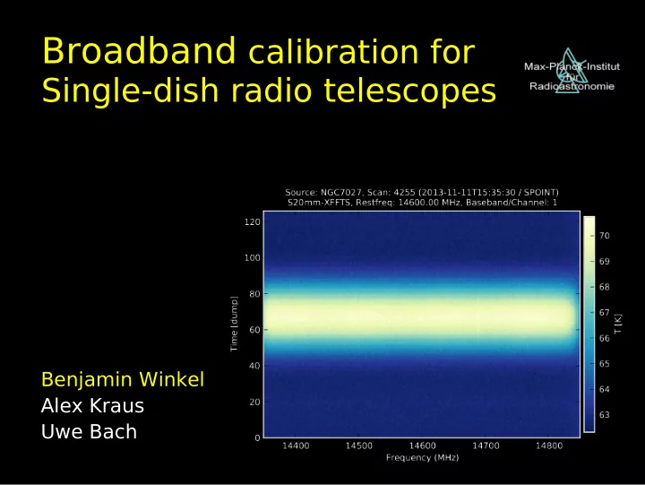
Broadband calibration for Single-dish radio telescopes Benjamin Winkel Alex Kraus Uwe Bach

Effelsberg: going broadband ● New receivers: – UBB (0.6 – 3.0 GHz) – C+ (4 – 9.3 GHz) – Ku (12 – 18 GHz) – K (18 – 26 GHz) – Q (33 – 50 GHz) ● New Backends: – 64k FFTS – Stacking: 1+M

Effelsberg: going broadband Calibration is frequency-dependent! Calibration is frequency-dependent!

Overview ● Motivation ● Introduction (continuum calibration) ● Spectroscopy calibration – Classic – Unbiased ● Conclusion / Outlook

Intro: fundamental equation

Intro: fundamental equation Calibrating a system means to determine G Calibrating a system means to determine G

Intro: continuum calibration ● Use known source (aka “calibrator”) to infer G

Intro: continuum calibration ● Use known source (aka “calibrator”) to infer G ● Problem: G is not perfectly stable

Intro: continuum calibration Gain variations Gain variations

Intro: continuum calibration ● Use known source (aka “calibrator”) to infer G ● Problem: G is not perfectly stable ● Solution: use a stable reference → Noise diode (T cal )

Solution: use a noise diode We now have It follows

Intro: using a noise diode We now have It follows This is really noisy, because

Solution: use a noise diode We now have It follows

Intro: noise diode + gain model We now have No averaging With averaging It follows

Intro: noise diode + gain model We now have No averaging With averaging It follows We still need to use a calibration source to infer T cal ! We still need to use a calibration source to infer T cal !

Spectroscopy: basics Again we have But now everything is a function of frequency

Spectroscopy: basics Again we have But now everything is a function of frequency Idea: Calibrate each spectral channel independently (using the same method as before)

Spectroscopy: basics Again we have As before, but vectorized

Spectroscopy: basics Again we have As before, but vectorized

Spectroscopy: basics Again we have As before, but vectorized Denominator is too small → numerically unstable

Spectroscopy: basics Again we have As before, but vectorized Average in time? → only possible if G is very stable Average in time? → only possible if G is very stable (long integration periods needed, because of small bandwidth per channel) (long integration periods needed, because of small bandwidth per channel) Average in frequency? → only possible if G is very flat Average in frequency? → only possible if G is very flat (usually not the case, especially not for ultra-wideband systems) (usually not the case, especially not for ultra-wideband systems)

Spectroscopy: position switching Observe O N and O FF -source

Spectroscopy: position switching Observe O N and O FF -source It follows

Spectroscopy: position switching Observe O N and O FF -source It follows But: T sys depends on time and frequency But: T sys depends on time and frequency → need to relate this to T cal again → need to relate this to T cal again

Spectroscopy: inferring T sys Observe O N and O FF -source Compute

Spectroscopy: inferring T sys Observe O N and O FF -source Compute This can be approximated by a constant (in frequency)! This can be approximated by a constant (in frequency)!

Spectroscopy: inferring T sys Observe O N and O FF -source Compute However, denominator is small → numerically unstable However, denominator is small → numerically unstable

Spectroscopy: classic solution “Classic” solution with

Spectroscopy: unbiased method Now switch to larger Now switch to larger bandwidth... bandwidth...

Spectroscopy: unbiased method Gauss-filtered Model this quantity and invert afterwards (avoids numerical instability)

Spectroscopy: unbiased method From mean Model this quantity and invert afterwards (avoids numerical instability) From Gauss-filtered

Spectroscopy: unbiased results

Spectroscopy: unbiased results Correct continuum signal!

Spectroscopy: unbiased results RRL: H109α

Spectroscopy: unbiased results RRL: H112α Classic method: line ratio systematically wrong!

Conclusion Need to incorporate frequency dependence Need to incorporate frequency dependence But But ● Modeling not always robust, may need supervision ● Modeling not always robust, may need supervision (e.g., in case of standing waves) (e.g., in case of standing waves) ● T sys may not be stable between O N and O FF ● T sys may not be stable between O N and O FF Weather can hurt a lot! Weather can hurt a lot! → Solution: cross-scanning → Solution: cross-scanning ● Frequency dependence also for opacity, ● Frequency dependence also for opacity, Elevation-gain curve, taper function Elevation-gain curve, taper function