SLIDE 1 Philippe Bonneton
EPOC/METHYS, CNRS, Bordeaux Univ.
5ième Ecole EGRIN – Institut d'Études Scientifiques de Cargèse, 29 mai - 2 juin 2017
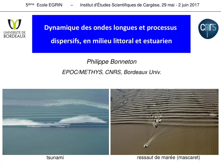
Dynamique des ondes longues et processus dispersifs, en milieu littoral et estuarien
tsunami ressaut de marée (mascaret)
SLIDE 2 Introduction Ondes longues z
d0
z = z(x,t) A0
0 c
2
d d A = =
λ
d0 , A0 , 0 𝑈0 0/ 𝑒0 = 𝑔(𝐵0/𝑒0, 𝑒0/0)
0<< 1
tsunamis, marées, ondes infragravitaires, ondes de crue, …
SLIDE 3 Introduction Ondes longues
Tissier , Bonneton et al., JCR2011
40 min 30 min 18 min 7 min
50 km a=2m dispersion
- ndes longues se propageant en milieu littoral et estuarien
fortes nonlinéarités dispersion
Formation et dynamique des chocs dispersifs
SLIDE 4 http://www.kohjumonline.com/anders.html
Sumatra 2004 tsunami reaching the coast of Thailand references:
- Grue et al. 2008
- Madsen et al. 2008
Introduction Tsunamis
SLIDE 5
Introduction Tsunamis
21st November 2016, Sunaoshi River in Tagajo city, Japan (earthquake 7.4)
SLIDE 6
Introduction Tsunamis
21st November 2016, Sunaoshi River in Tagajo city, Japan (earthquake 7.4)
SLIDE 7 Tsunamis, Arikawa et al. 2013
Impact on marine structures and buildings
Introduction Tsunamis
SLIDE 8 Introduction Tidal bore
Bonneton et al. JGR 2015
SLIDE 9 Introduction Tidal bore
Gironde estuary, Saint Pardon, Dordogne
https://vimeo.com/106090912, Jean-Marc Chauvet, Septembre 2014
SLIDE 10 Introduction Tidal bore
Sediment transport and erosion
Tidal Bore, Bonneton et al. 2015
SLIDE 11
Introduction Infragravity-wave
Costa Rica (video: Bonneton, P. 2012) wind waves (T0 10 s) infragravity waves (T0 1 min)
SLIDE 12
Urumea River – San Sebastian
Introduction Infragravity-wave
SLIDE 13 Introduction Plan
- 1. Introduction
- 2. Modèles d’onde longue
notions sur les effets dispersifs équations de Serre / Green-Naghdi applications : simulations numériques
- 3. Distorsion des ondes longues et formation de chocs
- 4. Dynamique des ressauts de marée et mascarets
Dynamique des ondes longues et processus dispersifs, en milieu littoral et estuarien
SLIDE 14
Introduction collaborations
Physical Oceanography Bonneton, N., Castelle, B., J-P., Sottolichio, A. (EPOC, Bordeaux) Frappart, F. (OMP, Toulouse) Martins K. (Bath Univ.) Tissier, M. (TU Delft) Long wave modeling Lannes, D. (IMB, Bordeaux) Ricchuito, M., Arpaia, L., Filippini, A. (INRIA, Bordeaux) Marche, F. (IMAG, Montpellier) Cienfuegos, R. (CIGIDEN, Chile), Barthélémy E. (LEGI, Grenoble)
SLIDE 15
notions sur les effets dispersifs équations de Serre / Green-Naghdi applications : simulations numériques
SLIDE 16
∂x + ∂w ∂z =
, ζ]
∂w ∂x − ∂u ∂z =
∂t + u ∂u ∂x + w ∂u ∂z = −
∂x ∂w ∂t + u ∂w ∂x + w ∂w ∂z = −g −
∂z P(z) = Patm z = ζ ∂ζ ∂t + u ∂ζ ∂x = w z = ζ w =
SLIDE 17
x′,
z = d
z′,
t =
λ
t′,
ζ = A
ζ′,
Φ = A
λ
Φ′,
P = ρ
gd P′.
SLIDE 18
∂x + ∂w ∂z =
∂w ∂x − ∂u ∂z =
∂t + ǫ
u ∂u
∂x + ǫ
∂z = −∂P ∂x ǫ∂w ∂t + ǫ
u ∂w
∂x + ǫ
∂z = − − ∂P ∂z P(z) = Patm z = ǫζ ∂ζ ∂t + ǫu ∂ζ ∂x =
z = ǫζ w =
SLIDE 19
exp
λ − t T )
exp (i(kx − ωt))
⇒ ω
= gk tanh(kd )
ζ(x, t) = A
exp
k t)
k = λ T
cφ = g k tanh(kd
)
λ
SLIDE 21
g k tanh(kd
)
≫
≫
g k
gλ
π
≪
≪
= (gd
) /
)
) )
cφ =
− µ k
SLIDE 23
−
∂x + ∂w ∂z
=
−
∂t + ǫ
u ∂u
∂x + ǫ
∂z + ∂P ∂x
=
∂t + ∂hU ∂x =
∂t + ǫ
U ∂U
∂x + ǫ
∂ ∂x ǫζ
−
(u
− U ) dz
−
∂ ∂x ǫζ
−
P dz
ǫζ
− u dz
SLIDE 24
∂t + ǫ
u ∂w
∂x + ǫ
∂z = − − ∂P ∂z
+ ǫΓ = −∂P
∂z Γ = ∂w
∂t + ǫu ∂w ∂x + ǫ µw ∂w ∂z
P = ǫζ − z + ǫ ǫζ
z
Γ dξ ǫζ
−
P dz =
+ ǫ
ǫζ
−
dz ǫζ
z
Γ dξ ǫζ
−
P dz =
+ ǫ
ǫζ
−
Γ(z +
) dz .
SLIDE 25
∂t + ∂hU ∂x =
∂t + ǫU ∂U ∂x + ∂ζ ∂x + ǫ h ∂ ∂x ǫζ
−
(u
− U ) dz
∂ ∂x ǫζ
−
(z +
)Γ dz
SLIDE 26
N
µjΦj . µ∂
Φ
∂x
+ ∂ Φ
∂z
=
Φ
+ µ
∂
Φ
+ ∂ Φ
.
Φ
=
(x, t) &
= Φ(z = ǫζ) = ψ(x, t) .
= −
) − h )∂ ψ
∂x
SLIDE 27
= ψ(x, t)
Φ
= −
) − h )∂ ψ
∂x
∂x = ∂ψ ∂x + µǫh∂ζ ∂x ∂
ψ
∂x
− µ ((z + ) − h )∂ ψ
∂x
+ O(µ )
U = ∂ψ ∂x + µǫh∂ζ ∂x ∂
ψ
∂x
+ µ ' h ∂ ψ
∂x
+ O(µ )
u = U − µ
(z + ) ∂ U
∂x
+ µ h ∂ U
∂x
+ O(µ )
w = ∂Φ ∂z = −µ(z +
)∂U
∂x + O(µ
)
SLIDE 28
= U − µ
(z + ) ∂ U
∂x
+ µ h ∂ U
∂x
+ O(µ )
w = ∂Φ ∂z = −µ(z +
)∂U
∂x + O(µ
)
∂ζ ∂t + ∂hU ∂x =
∂t + ǫU ∂U ∂x + ∂ζ ∂x + ǫ h ∂ ∂x ǫζ
−
(u
− U ) dz
−
∂ ∂x ǫζ
−
(z +
)Γ dz
−
(u
− U ) dz = O(µ )
Γ = −µ(z +
)
U
∂x∂t + ǫU ∂
U
∂x
− ǫ
∂U ∂x
SLIDE 29
∂t + ∂hU ∂x =
∂t + ǫU ∂U ∂x + ∂ζ ∂x = µ
'h
∂ ∂x
U
∂x∂t + ǫU ∂
U
∂x
− ǫ
∂U ∂x
)
) ǫ = O(µ)
) ǫ = O( )
+ ,
"
SLIDE 30
∂t + ∂U ∂x =
∂t + ∂ζ ∂x = µ
'
∂
U
∂
x∂t
cφ =
−/
− µk
SLIDE 31
+ A sech (K(x − Ct))
K =
+ ǫ )
= (gd
) / ( + ǫ ) /
= C(
− d
SLIDE 32 b(x,y)
Lannes and Bonneton (2009)
Long wave modelling 2D SGN
SLIDE 33 Bonneton, Chazel, Lannes, Marche and Tissier (2011) kd0 3
Reformulation of SGN equations
Long wave modelling 2D SGN
SLIDE 34
Lannes and Marche (2014) have proposed a new formulation where the operator to invert is time independent a considerable decrease of the computational time!
Long wave modelling 2D SGN
SLIDE 35 Numerical strategy: decoupling between the hyperbolic and the elliptic parts
e.g. Duran and Marche (2016), Filippini et al. (2017)
Strategy for wave breaking: description of broken-wave fronts as shocks by the NSWE, by skipping the dispersive step S2
Bonneton et al. (2011)
Long wave modelling 2D SGN
SLIDE 36 X (m)
NSWE S-GN S-GN S-GN
X (m) z (m)
Shoaling and breaking of regular waves over a sloping beach
Long wave modelling Applications
Tissier et al. (2012)
SLIDE 37 X (m) z (m)
Shoaling and breaking of regular waves over a sloping beach
Long wave modelling Applications
SLIDE 38 Experimental data Model prediction
L1 L2 L3 L4 L5 L6
Breaking point
Validation with Cox (1995) experiments Shoaling and breaking of regular waves over a sloping beach
Long wave modelling Applications
SLIDE 39 Truc Vert Beach 2001 Offshore wave conditions: 0°, Hs=3 m, Ts=12 s Maximum surf zone width: 500 m Bottom topography and pressure sensor locations
Comparison with field data
Long wave modelling Applications
SLIDE 40 1 2 3 4 5 6 7 8
Validation with Beji and Battjes (1993) experiments Periodic waves breaking over a bar
Long wave modelling Applications
Tissier et al. (2012)
SLIDE 41
Validation with Beji and Battjes (1993) experiments Periodic waves breaking over a bar
Long wave modelling Applications
Tissier et al. (2012)
SLIDE 42 1 2 3 4 5 6 7 8
Validation with Beji and Battjes (1993) experiments
Laboratory data Model prediction
Long wave modelling Applications
Tissier et al. (2012)
SLIDE 43 8 9 10 11 12 13 14 15
Wave overtopping and multiple shorelines Solitary waves overtopping a seawall (Hsiao and Lin, 2010)
Long wave modelling Applications
SLIDE 44
Wave overtopping and multiple shorelines Hsiao et Lin (2010) COBRAS model 2D VOF model RANS equations K- SURF-GN
Long wave modelling Applications
SLIDE 45 Wave overtopping and multiple shorelines
BARDEX II (HYDRALAB project, Delta Flumes, PI: Gerd Masselink) Barrier Dynamics Experiment : shallow water sediment transport processes in the inner surf, swash and overwash zone.
Long wave modelling Applications
SLIDE 46 Wave overtopping and multiple shorelines
BARDEX II (HYDRALAB project, Delta Flumes, PI: Gerd Masselink) Barrier Dynamics Experiment : shallow water sediment transport processes in the inner surf, swash and overwash zone.
Long wave modelling Applications
SLIDE 47
Marche et Lannes, 2014
Long wave modelling Applications
SLIDE 48 Undular bore (dispersive choc)
Data from Soares-Frazao et Zech (2002), Fr = 1.104
Long wave modelling Applications
SLIDE 49
- 3. Distorsion des ondes longues et formation de chocs
SLIDE 50 tsunami bore tidal bore
What are the conditions for tsunami-like bore formation in coastal and estuarine environments? Basic conditions for bore formation
SLIDE 51 Basic conditions for bore formation
4000 m
deep
D0 =150 m
Continental shelf Lc
- the continental shelf is relatively flat
Bore inception ?
𝑴w0 = 𝒉D0 0
SLIDE 52
Basic conditions for bore formation 0 << 1 0 =O(1)
SLIDE 53 Basic conditions for bore formation 0 << 1 0 =O(1)
40 min 30 min 18 min 7 min
50 km a=2m Serre Green Naghdi model
Tissier , Bonneton et al., JCR2011
SLIDE 54 Basic conditions for bore formation 0 << 1 0 =O(1)
40 min 30 min 18 min 7 min
50 km a=2m Serre Green Naghdi model
Tissier , Bonneton et al., JCR2011
SLIDE 55
Basic conditions for bore formation
SLIDE 56 Basic conditions for bore formation
x
t=ts t=0 t=3ts/4 t=ts/2 t=ts/4
xs
SLIDE 57 Basic conditions for bore formation
4000 m
deep
Continental shelf Lc
see Madsen et al 2008
D0 =150 m
SLIDE 58 Basic conditions for bore formation
4000 m
deep
150 m
Continental shelf Lc
SLIDE 59 Basic conditions for bore formation
4000 m
deep
150 m
Continental shelf Lc
SLIDE 60 4000 m
deep
150 m
Continental shelf Lc Continental shelves D0 150 m
- tsunamis: A0 2 m, T0 25 min xs = 460 km
- tides: T0 744 min xs >> Lc
no tidal bore
Basic conditions for bore formation
SLIDE 61 4000 m
deep
150 m
Continental shelf Lc
- tsunamis: bores may occur in large and shallow (few tens of m) coastal environments:
marine coastal plains (e.g.: deltas, alluvial estuaries) or carbonate platforms (e.g.: coral reef systems)
Basic conditions for bore formation
SLIDE 62 4000 m
deep
150 m
Continental shelf Lc
- tsunamis: bores may occur in large and shallow (few tens of m) coastal environments:
marine coastal plains (e.g.: deltas, alluvial estuaries) or carbonate platforms (e.g.: coral reef systems)
- tides: bores can occur in long shallow alluvial estuaries
L 100 km D0 10 m
Basic conditions for bore formation
SLIDE 63 4000 m
deep
150 m
Continental shelf Lc
Basic conditions for bore formation
in such shallow environments friction can play a significant role
- tsunamis: bores may occur in large and shallow (few tens of m) coastal environments:
marine coastal plains (e.g.: deltas, alluvial estuaries) or carbonate platforms (e.g.: coral reef systems)
- tides: bores can occur in long shallow alluvial estuaries
SLIDE 64
- 4. Dynamique des ressauts de marée et mascarets
SLIDE 65 Conditions for tidal bore formation Worldwide tidal bores
Severn River - England Qiantang River – China Kampar River – Sumatra (Bono) Amazon River – Brazil (Pororoca)
SLIDE 66 Large amplitude spring tide – 10th September 2010
Bonneton et al. JGR 2015
Conditions for tidal bore formation Worldwide tidal bores
SLIDE 67 Conditions for tidal bore formation Worldwide tidal bores
Gironde/Garonne/Dordogne estuary – France 3 field campaigns : a unique long-term high-frequency database
SLIDE 68 Conditions for tidal bore formation Worldwide tidal bores
Bonneton et al. JGR 2015 Gironde/Garonne/Dordogne estuary – France 3 field campaigns : a unique long-term high-frequency database
SLIDE 69
Conditions for tidal bore formation Physical criteria
Scaling analysis
Large tidal range (Tr0=2A0) Small water depth Large-scale funnel-shaped estuaries
Chanson (2012) : Tr0 > 4.5-6 m coastal plain alluvial estuaries
SLIDE 70 Conditions for tidal bore formation Physical criteria
Scaling analysis
Large tidal range Small water depth Large-scale funnel-shaped estuaries
coastal plain alluvial estuaries
Identify the characteristic scales of the problem:
- morphology of alluvial estuaries
- tidal waves
SLIDE 71 Scheldt estuary Savenije 2012
Conditions for tidal bore formation Alluvial estuary morphology
along-channel coordinate
Tide-dominated alluvial estuaries show many morphological similarities all over the world
SLIDE 72
Pungue estuary Graas et al. 2008
Conditions for tidal bore formation Alluvial estuary morphology
SLIDE 73 𝐶 = 𝐶0𝑓−
𝑦 𝑀𝐶0
- Lb0 : convergence length
- D0 : characteristic water depth
Conditions for tidal bore formation Alluvial estuary morphology
SLIDE 74
𝑀𝑥0 = 𝐸0/0
- A0=Tr0/2 (mean spring tidal amplitude)
Conditions for tidal bore formation Scaling analysis
SLIDE 75
- Lb0
- D0
- T0=12.4 h
- A0=Tr0/2
- Cf0 : friction coefficient
- Q0 : freshwater discharge
Conditions for tidal bore formation Scaling analysis
SLIDE 76
- Lb0
- D0
- T0=12.4 h
- A0=Tr0/2
- Cf0 : friction coefficient
5 external variables Conditions for tidal bore formation Scaling analysis
SLIDE 77
Conditions for tidal bore formation Scaling analysis
SLIDE 78
Conditions for tidal bore formation Scaling analysis
SLIDE 79 Conditions for tidal bore formation Scaling analysis
𝐸𝑗 =
𝐷𝑔0𝑀𝑐0𝐵0 𝐸02
> 1.5
K 1, for tidal bore estuaries
Bonneton et al., JGR 2015
necessary condition for tidal bore formation by not a sufficient one
SLIDE 80 Conditions for tidal bore formation Scaling analysis
explore the 3D dimensionless external parameter space: (0 , 0 , 0)
- Field data: 21 convergent alluvial estuaries
Bonneton, P., Filippini, A.G., Arpaia, L., Bonneton, N. and Ricchiuto, M 2016. Conditions for tidal bore formation in convergent alluvial estuaries. ECSS, 172, 121-127
- Numerical simulations: 225 runs of a shallow water model
Filippini, A.G., Arpaia, L., Bonneton, P., and Ricchiuto, M. 2017. Modelling analysis of tidal bore formation in convergent estuaries. in revision
SLIDE 81 1 Chao Phya Thailand 2 Columbia USA 3 Conwy UK 4 Corantijn USA 5 Daly Australia 6 Delaware USA 7 Elbe Germany 8 Gironde France 9 Hooghly India 10 Humber UK 11 Limpopo Mozambique 12 Loire France 13 Mae Klong Thailand 14 Maputo Mozambique 15 Ord Australia 16 Pungue Mozambique 17 Qiantang China 18 Scheldt Netherlands 19 Severn UK 20 Tha Chin Thailand 21 Thames UK
- 21 convergent alluvial estuaries
- 9 tidal bore estuaries
Conditions for tidal bore formation Field data
D0, Lb0, A0=Tr0/2 , Cf0
SLIDE 82 Conditions for tidal bore formation Field data
Tidal bore estuaries: 0 2.4 2D parameter space (0 , 0)
1 Chao Phya Thailand 2 Columbia USA 3 Conwy UK 4 Corantijn USA 5 Daly Australia 6 Delaware USA 7 Elbe Germany 8 Gironde France 9 Hooghly India 10 Humber UK 11 Limpopo Mozambique 12 Loire France 13 Mae Klong Thailand 14 Maputo Mozambique 15 Ord Australia 16 Pungue Mozambique 17 Qiantang China 18 Scheldt Netherlands 19 Severn UK 20 Tha Chin Thailand 21 Thames UK
SLIDE 83 Conditions for tidal bore formation Field data
Tidal bores occur when 0 > c(0)
c(0)
1 Chao Phya Thailand 2 Columbia USA 3 Conwy UK 4 Corantijn USA 5 Daly Australia 6 Delaware USA 7 Elbe Germany 8 Gironde France 9 Hooghly India 10 Humber UK 11 Limpopo Mozambique 12 Loire France 13 Mae Klong Thailand 14 Maputo Mozambique 15 Ord Australia 16 Pungue Mozambique 17 Qiantang China 18 Scheldt Netherlands 19 Severn UK 20 Tha Chin Thailand 21 Thames UK
SLIDE 84
Numerical investigation of the 2D parameter space (0 , 0)
225 runs with 0 = 2 Conditions for tidal bore formation Numerical simulations
Filippini, A.G., Arpaia, L., Bonneton, P., and Ricchiuto, M. 2017
SLIDE 85 Conditions for tidal bore formation Numerical simulations
SGN / SV
Filippini et al. 2017
SLIDE 86 Conditions for tidal bore formation Numerical simulations
Filippini et al. 2017
SGN / SV
SLIDE 87 Numerical investigation of the 2D parameter space (0 , 0)
225 runs with 0 = 2 Conditions for tidal bore formation Numerical simulations
2D nonlinear shallow water model developed by Ricchiuto, JCP 2015
- shock capturing residual distribution scheme
- 2nd order in space and time
- unstructured grids suitable for real estuarine applications
Filippini et al. 2017
SLIDE 88 Conditions for tidal bore formation Numerical simulations
𝑇𝑛𝑏𝑦 = 𝑛𝑏𝑦 𝜖 𝜖𝑦
- ne example on the 225 runs
Filippini et al. 2017
SLIDE 89 Conditions for tidal bore formation Numerical simulations 0 = 2
𝑇𝑛𝑏𝑦 𝑇𝑛𝑏𝑦 Filippini et al. 2017
SLIDE 90 Conditions for tidal bore formation Numerical simulations
Filippini et al. 2017
𝑈𝑠 = 𝑈𝑠 𝑀𝑑 − 𝑈𝑠(0) 𝑈𝑠(0)
rate of change of the tidal range
Theoretical zero-amplification curve:
(Savenije et al. 2008)
00 = 0(0
2 + 1)
damping amplification
SLIDE 91
Conditions for tidal bore formation Estuary classification
Tidal bores occur when 0 > c(0)
c(0)
SLIDE 92 Conclusion
tsunami ressaut de marée (mascaret)
Ondes longues et chocs dispersifs
SLIDE 93 25 km
Large scale phenomenon tidal wave Small scale wave phenomenon tidal bore
- LTW 100 km
- TTW 12.4 h
- LTB 10 m
- TTB 1 s
Conclusion
SLIDE 94
Conclusion
SLIDE 95
Thank you for your attention