
SLIDE 1
Dynamic Programming
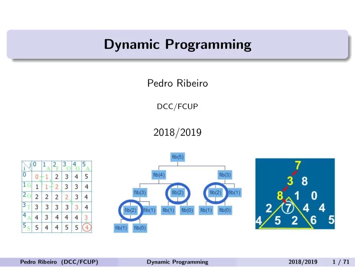
Pedro Ribeiro
DCC/FCUP
2018/2019
Pedro Ribeiro (DCC/FCUP) Dynamic Programming 2018/2019 1 / 71
Dynamic Programming Pedro Ribeiro DCC/FCUP 2018/2019 Pedro - - PowerPoint PPT Presentation
Dynamic Programming Pedro Ribeiro DCC/FCUP 2018/2019 Pedro Ribeiro (DCC/FCUP) Dynamic Programming 2018/2019 1 / 71 Fibonacci Numbers Probably the most famous number sequence , defined by Leonardo Fibonacci 0,1,1,2,3,5,8,13,21,34,...
Pedro Ribeiro
DCC/FCUP
2018/2019
Pedro Ribeiro (DCC/FCUP) Dynamic Programming 2018/2019 1 / 71
Probably the most famous number sequence, defined by Leonardo Fibonacci
Fibonacci Numbers F(0) = 0 F(1) = 1 F(n) = F(n − 1) + F(n − 2)
Pedro Ribeiro (DCC/FCUP) Dynamic Programming 2018/2019 2 / 71
How to implement? Implementing directly from the definition: Fibonacci (from the definition) fib(n): If n = 0 or n = 1 then return n Else return fib(n − 1) + fib(n − 2) Negative points of this implementation?
Pedro Ribeiro (DCC/FCUP) Dynamic Programming 2018/2019 3 / 71
Computing fib(5):
Pedro Ribeiro (DCC/FCUP) Dynamic Programming 2018/2019 4 / 71
Computing fib(5): For instance, fib(2) is called 3 times!
Pedro Ribeiro (DCC/FCUP) Dynamic Programming 2018/2019 5 / 71
How to improve?
◮ Start from zero and keep in memory the last two numbers of the
sequence
Fibonacci (more efficient iterative version) fib(n): If n = 0 or n = 1 then return n Else f1 ← 1 f2 ← 0 For i ← 2 to n do f ← f1 + f2 f2 ← f1 f1 ← f return f
Pedro Ribeiro (DCC/FCUP) Dynamic Programming 2018/2019 6 / 71
Concepts to recall:
◮ Dividing a problem in subproblems of the same type ◮ Calculating the same subproblem just once
Can these ideas be used in more ”complicated” problems?
Pedro Ribeiro (DCC/FCUP) Dynamic Programming 2018/2019 7 / 71
”Classic” problem from the 1994 International Olympiad in Informatics Compute the path, starting on the top of the pyramid and ending on the base, with the biggest sum. In each step we can go diagonally down and left or down and right.
Pedro Ribeiro (DCC/FCUP) Dynamic Programming 2018/2019 8 / 71
Two possible paths: Constraints: all the numbers are integers between 0 and 99 and the number of lines in the pyramid is at most 100.
Pedro Ribeiro (DCC/FCUP) Dynamic Programming 2018/2019 9 / 71
How to solve the problem? Idea: Exhaustive search (aka ”Brute Force”)
◮ Evaluate all the paths and choose the best one.
How much time does this take? How many paths exist? Analysing the temporal complexity:
◮ In each line we can take one of two decisions: left or right ◮ Let n be the height of the pyramid. A path corresponds to... n − 1
decisions!
◮ There are 2n−1 different paths ◮ A program to compute all possible paths has therefore complexity
O(2n): exponential!
◮ 299 ∼ 6.34 × 1029 (633825300114114700748351602688) Pedro Ribeiro (DCC/FCUP) Dynamic Programming 2018/2019 10 / 71
When we are at the top we have two possible choices (left or right): In each case, we need to have in account all possible paths of the respective subpyramid.
Pedro Ribeiro (DCC/FCUP) Dynamic Programming 2018/2019 11 / 71
But what do we really need to know about these subpyramids? The only thing that matters is the best internal path, which is a smaller instance of the same problem! For the example, the solution is 7 plus the maximum between the value of the best paths in each subpyramid
Pedro Ribeiro (DCC/FCUP) Dynamic Programming 2018/2019 12 / 71
This problem can then be solved recursively
◮ Let P[i][j] be the j-th number of the i-th line ◮ Let Max(i, j) be the best we can do from position (i, j)
1 2 3 4 5 1 7 2 3 8 3 8 1 4 2 7 4 4 5 4 5 2 6 5
Pedro Ribeiro (DCC/FCUP) Dynamic Programming 2018/2019 13 / 71
Number Pyramid (from the recursive definition) Max(i, j): If i = n then return P[i][j] Else return P[i][j] + maximum (Max(i + 1, j), Max(i + 1, j + 1)) To solve the problem we just need to call... Max(1,1) 1 2 3 4 5 1 7 2 3 8 3 8 1 4 2 7 4 4 5 4 5 2 6 5
Pedro Ribeiro (DCC/FCUP) Dynamic Programming 2018/2019 14 / 71
We still have exponential growth! We are evaluating the same problem several times...
Pedro Ribeiro (DCC/FCUP) Dynamic Programming 2018/2019 15 / 71
We need to reuse what we have already computed
◮ Compute only once each subproblem
Idea: create a table with the value we got for each subproblem
◮ Matrix M[i][j]
Is there an order to fill the table so that when we need a value we have already computed it?
Pedro Ribeiro (DCC/FCUP) Dynamic Programming 2018/2019 16 / 71
We can start from the end! (pyramid base)
Pedro Ribeiro (DCC/FCUP) Dynamic Programming 2018/2019 17 / 71
We can start from the end! (pyramid base)
Pedro Ribeiro (DCC/FCUP) Dynamic Programming 2018/2019 18 / 71
We can start from the end! (pyramid base)
Pedro Ribeiro (DCC/FCUP) Dynamic Programming 2018/2019 19 / 71
We can start from the end! (pyramid base)
Pedro Ribeiro (DCC/FCUP) Dynamic Programming 2018/2019 20 / 71
Having in mind the way we fill the table, we can even reuse P[i][j]: Number Pyramid (polynomial solution) Compute(): For i ← n − 1 to 1 do For j ← 1 to i do P[i][j] ← P[i][j] + maximum (P[i + 1][j], P[i + 1][j + 1]) With this the solution is in... P[1][1] Now the time needed to solve the problem only grows polynomially (O(n2)) and we have an admissible solution for the problem (992 = 9801)
Pedro Ribeiro (DCC/FCUP) Dynamic Programming 2018/2019 21 / 71
What if we need to know what are the numbers in the best path? We can use the computed table!
Pedro Ribeiro (DCC/FCUP) Dynamic Programming 2018/2019 22 / 71
To solve the number pyramid number we used...
Pedro Ribeiro (DCC/FCUP) Dynamic Programming 2018/2019 23 / 71
Dynamic Programming An algorithmic technique, typically used in optimization problems, which is based on storing the results of subproblems instead of recomputing them. Algorithmic Technique: general method for solving problem that have some common characteristics Optimization Problem: find the ”best” solution among all possible solutions, according to a certain criteria (goal function). Normally it means finding a minimum or a maximum.
Classic trade of space for time
Pedro Ribeiro (DCC/FCUP) Dynamic Programming 2018/2019 24 / 71
What are then the characteristics that a problem must present so that it can be solved using DP?
Pedro Ribeiro (DCC/FCUP) Dynamic Programming 2018/2019 25 / 71
Optimal substructure When the optimal solution of a problem contains in itself solutions for subproblems of the same type Example On the number pyramid number problem, the optimal solution contains in itself optimal solutions for subpyramids If a problem presents this characteristic, we say that it respects the
Pedro Ribeiro (DCC/FCUP) Dynamic Programming 2018/2019 26 / 71
Be careful! Not all problems present optimal substructure! Example without optimal substructure Imagine that in the problem of the number pyramid the goal is to find the path that maximizes the remainder of the integer division between the sum
The optimal solution (1 → 5 → 5) does not contain the optimal solution for the subpyramid shown (5 → 4)
Pedro Ribeiro (DCC/FCUP) Dynamic Programming 2018/2019 27 / 71
Overlapping Subproblems When the search space is ”small”, that is, there are not many subproblems to solve because many subproblems are essentially equal. Example In the problem of the number pyramid, for a certain problem instance, there are only n + (n − 1) + ... + 1 < n2 subproblems because, as we have seen, many subproblems are coincident
Pedro Ribeiro (DCC/FCUP) Dynamic Programming 2018/2019 28 / 71
Be careful! This characteristic is also not always present. Even with overlapping subproblems there are too many subproblems to solve
There is no overlap between subproblems Examplo In MergeSort, each recursive call is made to a new subproblem, different from all the others.
Pedro Ribeiro (DCC/FCUP) Dynamic Programming 2018/2019 29 / 71
If a problem presents these two characteristics, we have a good hint that DP is applicable. What steps should we then follow to solve a problem with DP? Guide to solve with DP
1
Characterize the optimal solution of the problem
2
Recursively define the optimal solution, by using optimal solutions
3
Compute the solutions of all subproblems: bottom-up or top-down
4
Reconstruct the optimal solution, based on the computed values (optional - only if necessary)
Pedro Ribeiro (DCC/FCUP) Dynamic Programming 2018/2019 30 / 71
1) Characterize the optimal solution of the problem
Really understand the problem Verify if an algorithm that verifies all solutions (brute force) is not enough Try to generalize the problem (it takes practice to understand how to correctly generalize) Try to divide the problem in subproblems of the same type Verify if the problem obeys the optimality principle Verify if there are overlapping subproblems
Pedro Ribeiro (DCC/FCUP) Dynamic Programming 2018/2019 31 / 71
2) Recursively define the optimal solution, by using optimal solutions of subproblems
Recursively define the optimal solution value, exactly and with rigour, from the solutions of subproblems of the same type Imagine that the values of optimal solutions are already available when we need them No need to code. You can just mathematically define the recursion
Pedro Ribeiro (DCC/FCUP) Dynamic Programming 2018/2019 32 / 71
3) Compute the solutions of all subproblems: bottom-up
Find the order in which the subproblems are needed, from the smaller subproblem until we reach the global problem and implement, using a table Usually this order is the inverse to the normal order of the recursive function that solves the problem Normal solving order +---------+
+-----+ |Beginning| | End | +---------+ <-------------- +-----+ Order when using DP
Pedro Ribeiro (DCC/FCUP) Dynamic Programming 2018/2019 33 / 71
3) Compute the solutions of all subproblems: top-down
There is a technique, known as ”memoization”, that allows us to solve the problem by the normal order. Just use the recursive function directly obtained from the definition
When we need to access a value for the first time we need to compute it, and from then on we just need to see the already computed result.
Pedro Ribeiro (DCC/FCUP) Dynamic Programming 2018/2019 34 / 71
4) Reconstruct the optimal solution, based on the computed values
It may (or may not) be needed, given what the problem asks for Two alternatives:
◮ Directly from the subproblems table ◮ New table that stores the decisions in each step
If we do not need to know the solution in itself, we can eventually save some space
Pedro Ribeiro (DCC/FCUP) Dynamic Programming 2018/2019 35 / 71
Given a number sequence:
Compute the longest increasing subsequence (not necessarily contiguous)
Pedro Ribeiro (DCC/FCUP) Dynamic Programming 2018/2019 36 / 71
1) Characterize the optimal solution of the problem
Let n be the size of the sequence and num[i] the i-th number ”Brute force”, how many options? Exponential! Generalize and solve with subproblems of the same type:
◮ Let best(i) be the size of the best subsequence starting from the i-th
position
◮ Base case: the best subsequence from the last position has size... 1! ◮ General case: for a given i, we can continue to all numbers from i + 1
to n, as long as they are... bigger or equal
⋆ For those numbers, we only need to know the best starting from them!
(optimality principle)
⋆ The best, starting from a position, is necessary for computing all the
positions of lower index! (overlapping subproblems)
Pedro Ribeiro (DCC/FCUP) Dynamic Programming 2018/2019 37 / 71
2) Recursively define the optimal solution, by using optimal solutions of subproblems
n - sequence size num[i] - number in position i best(i) - size of best sequence starting in position i Recursive Solution for LIS Problem best(n) = 1 best(i) = 1 + max{best(j): i < j ≤ n, num[j] > num[i]} for 1 ≤ i < n
Pedro Ribeiro (DCC/FCUP) Dynamic Programming 2018/2019 38 / 71
3) Compute the solutions of all subproblems: bottom-up
Let best[] the table to save the values of best() LIS Problem - O(n2) Compute(): best[n] ← 1 For i ← n − 1 to 1 do best[i] ← 1 For j ← i + 1 to n do If num[j] > num[i] and 1 + best[j] > best[i] then best[i] ← 1 + best[j] i 1 2 3 4 5 6 7 8 9 10 num[i] 7 6 10 3 4 1 8 9 5 2 best[i] 3 3 1 4 3 3 2 1 1 1
Pedro Ribeiro (DCC/FCUP) Dynamic Programming 2018/2019 39 / 71
4) Reconstruct the optimal solution
We will exemplify with an auxiliary table that stores the decisions Let next[i] be the next position in order to obtain the best solution from position i (’X’ if it is the last position of the solution). i 1 2 3 4 5 6 7 8 9 10 num[i] 7 6 10 3 4 1 8 9 5 2 best[i] 3 3 1 4 3 3 2 1 1 1 next[i] 7 7 X 5 7 7 8 X X X
Pedro Ribeiro (DCC/FCUP) Dynamic Programming 2018/2019 40 / 71
LIS Problem - O(n2) Compute(): best[n] ← 1 For i ← n − 1 to 1 do best[i] ← 1 For j ← i + 1 to n do If num[j] > num[i] and 1 + best[j] > best[i] then best[i] ← 1 + best[j] We can change the second loop and transform it into binary search
Pedro Ribeiro (DCC/FCUP) Dynamic Programming 2018/2019 41 / 71
Let index(i) be the index k of the largest value num[k] such that exists an increasing sequence of length i starting in that position k Let index[] be a table storing those values: i 1 2 3 4 5 6 7 8 9 10 num[i] 7 6 10 3 4 1 8 9 5 2 best[i] 3 3 1 4 3 3 2 1 1 1 index[i] 10 num[index[i]] 2 At each of our n iterations we can just binary search on num[index[i]] for the best continuation our current value
Pedro Ribeiro (DCC/FCUP) Dynamic Programming 2018/2019 42 / 71
Let index(i) be the index k of the largest value num[k] such that exists an increasing sequence of length i starting in that position k Let index[] be a table storing those values: i 1 2 3 4 5 6 7 8 9 10 num[i] 7 6 10 3 4 1 8 9 5 2 best[i] 3 3 1 4 3 3 2 1 1 1 index[i] 9 num[index[i]] 5 At each of our n iterations we can just binary search on num[index[i]] for the best continuation our current value
Pedro Ribeiro (DCC/FCUP) Dynamic Programming 2018/2019 43 / 71
Let index(i) be the index k of the largest value num[k] such that exists an increasing sequence of length i starting in that position k Let index[] be a table storing those values: i 1 2 3 4 5 6 7 8 9 10 num[i] 7 6 10 3 4 1 8 9 5 2 best[i] 3 3 1 4 3 3 2 1 1 1 index[i] 8 num[index[i]] 9 At each of our n iterations we can just binary search on num[index[i]] for the best continuation our current value
Pedro Ribeiro (DCC/FCUP) Dynamic Programming 2018/2019 44 / 71
Let index(i) be the index k of the largest value num[k] such that exists an increasing sequence of length i starting in that position k Let index[] be a table storing those values: i 1 2 3 4 5 6 7 8 9 10 num[i] 7 6 10 3 4 1 8 9 5 2 best[i] 3 3 1 4 3 3 2 1 1 1 index[i] 8 7 num[index[i]] 9 8 At each of our n iterations we can just binary search on num[index[i]] for the best continuation our current value
Pedro Ribeiro (DCC/FCUP) Dynamic Programming 2018/2019 45 / 71
Let index(i) be the index k of the largest value num[k] such that exists an increasing sequence of length i starting in that position k Let index[] be a table storing those values: i 1 2 3 4 5 6 7 8 9 10 num[i] 7 6 10 3 4 1 8 9 5 2 best[i] 3 3 1 4 3 3 2 1 1 1 index[i] 8 7 6 num[index[i]] 9 8 1 At each of our n iterations we can just binary search on num[index[i]] for the best continuation our current value
Pedro Ribeiro (DCC/FCUP) Dynamic Programming 2018/2019 46 / 71
Let index(i) be the index k of the largest value num[k] such that exists an increasing sequence of length i starting in that position k Let index[] be a table storing those values: i 1 2 3 4 5 6 7 8 9 10 num[i] 7 6 10 3 4 1 8 9 5 2 best[i] 3 3 1 4 3 3 2 1 1 1 index[i] 8 7 5 num[index[i]] 9 8 4 At each of our n iterations we can just binary search on num[index[i]] for the best continuation our current value
Pedro Ribeiro (DCC/FCUP) Dynamic Programming 2018/2019 47 / 71
Let index(i) be the index k of the largest value num[k] such that exists an increasing sequence of length i starting in that position k Let index[] be a table storing those values: i 1 2 3 4 5 6 7 8 9 10 num[i] 7 6 10 3 4 1 8 9 5 2 best[i] 3 3 1 4 3 3 2 1 1 1 index[i] 8 7 5 4 num[index[i]] 9 8 4 3 At each of our n iterations we can just binary search on num[index[i]] for the best continuation our current value
Pedro Ribeiro (DCC/FCUP) Dynamic Programming 2018/2019 48 / 71
Let index(i) be the index k of the largest value num[k] such that exists an increasing sequence of length i starting in that position k Let index[] be a table storing those values: i 1 2 3 4 5 6 7 8 9 10 num[i] 7 6 10 3 4 1 8 9 5 2 best[i] 3 3 1 4 3 3 2 1 1 1 index[i] 3 7 5 4 num[index[i]] 10 8 4 3 At each of our n iterations we can just binary search on num[index[i]] for the best continuation our current value
Pedro Ribeiro (DCC/FCUP) Dynamic Programming 2018/2019 49 / 71
Let index(i) be the index k of the largest value num[k] such that exists an increasing sequence of length i starting in that position k Let index[] be a table storing those values: i 1 2 3 4 5 6 7 8 9 10 num[i] 7 6 10 3 4 1 8 9 5 2 best[i] 3 3 1 4 3 3 2 1 1 1 index[i] 3 7 2 4 num[index[i]] 10 8 6 3 At each of our n iterations we can just binary search on num[index[i]] for the best continuation our current value
Pedro Ribeiro (DCC/FCUP) Dynamic Programming 2018/2019 50 / 71
Let index(i) be the index k of the largest value num[k] such that exists an increasing sequence of length i starting in that position k Let index[] be a table storing those values: i 1 2 3 4 5 6 7 8 9 10 num[i] 7 6 10 3 4 1 8 9 5 2 best[i] 3 3 1 4 3 3 2 1 1 1 index[i] 3 7 1 4 num[index[i]] 10 8 7 3 At each of our n iterations we can just binary search on num[index[i]] for the best continuation our current value
Pedro Ribeiro (DCC/FCUP) Dynamic Programming 2018/2019 51 / 71
Let index(i) be the index k of the largest value num[k] such that exists an increasing sequence of length i starting in that position k Let index[] be a table storing those values: i 1 2 3 4 5 6 7 8 9 10 num[i] 7 6 10 3 4 1 8 9 5 2 best[i] 3 3 1 4 3 3 2 1 1 1 index[i] 3 7 1 4 num[index[i]] 10 8 7 3 At each of our n iterations we can just binary search on num[index[i]] for the best continuation our current value Each of the n iterations takes log n (one binary search), and so our total complexity is O(n log n)
Pedro Ribeiro (DCC/FCUP) Dynamic Programming 2018/2019 52 / 71
0-1 Knapsack Problem Input: A backpack of capacity C A set of n materials, each one with weight wi and value vi Output: The allocation of materials to the backpack that maximizes the transported value. The materials cannot be ”broken” in smaller pieces, that is, for a given material i we can either take it all (xi = 1) or we leave it all (xi = 0) What we want is therefore to obey the following constraints The materials fit in the backpack (
i
xiwi ≤ C) The value transported is the maximum possible (maximize
i
xivi)
Pedro Ribeiro (DCC/FCUP) Dynamic Programming 2018/2019 53 / 71
A greedy solution will not work on this integer case Input Example Input: 5 objects and C = 11 i 1 2 3 4 5 wi 1 2 5 6 7 vi 1 6 18 22 28 vi/wi 1 3 3.6 3.66 4
◮ Choosing max ratio first will result in {1, 2, 7} with a value of 35 ◮ Choosing max value first will also result in {1, 2, 7} with a value of 35 ◮ Choosing min weight first will result in {1, 2, 5} with a value of 25 ◮ ... ◮ None of these is optimal: we could get a value of 40 with {3, 4} Pedro Ribeiro (DCC/FCUP) Dynamic Programming 2018/2019 54 / 71
1) Characterize the optimal solution of the problem
”Brute force”, how many options? Exponential (2n)! Let’s first consider the unbounded case (no limit on number of items of each type) In this unbounded case we could generalize in the following way:
◮ Let best(i) be the best value we can get for capacity i ◮ Base case: best(0) = 0 (obviously) ◮ General case: for a given i, we can simple see all possible items and
get the best if we insert that item: best(i) = max (vj + best(i − wj) : 1 ≤ j ≤ n, wj ≤ i) for 1 ≤ i ≤ C
But how can we limit the amount of items of each type?
Pedro Ribeiro (DCC/FCUP) Dynamic Programming 2018/2019 55 / 71
1) Characterize the optimal solution of the problem
Let’s add more information to our DP state
◮ Let best(i, j) be the best value we can get for capacity j using only the
first i materials
◮ For computing the values of a given best(i, j) we can now simply use
the values of previously computed best(i − 1, k)
◮ Let’s put all the pieces into place... Pedro Ribeiro (DCC/FCUP) Dynamic Programming 2018/2019 56 / 71
2) Recursively define the optimal solution
n - number of materials wi - weight of material i vi - value of material of material i C - capacity of backpack best(i,j) - maximum possible value for capacity j using the first i materials Recursive Solution for 0-1 Knapsack best(0, j) = 0 for 0 ≤ j ≤ C best(i, j) = best(i − 1, j) if (wi > j) best(i, j) = max {best(i − 1, j), best(i − 1, j − wi) + vi} if (wi ≤ j) for 1 ≤ i ≤ n, 0 ≤ j ≤ C The desired result is: best(n,C)
Pedro Ribeiro (DCC/FCUP) Dynamic Programming 2018/2019 57 / 71
Let’s see a table of results to better understand the DP formulation: Input Example Input: n = 5 and C = 11 i 1 2 3 4 5 wi 1 2 5 6 7 vi 1 6 18 22 28 Capacity Items 1 2 3 4 5 6 7 8 9 10 11 {} {1} 1 1 1 1 1 1 1 1 1 1 1 {1,2} 1 6 7 7 7 7 7 7 7 7 7 {1,2,3} 1 6 7 7 18 19 24 25 25 25 25 {1,2,3,4} 1 6 7 7 18 22 24 28 29 29 40 {1,2,3,4,5} 1 6 7 7 18 22 28 39 34 35 40
Pedro Ribeiro (DCC/FCUP) Dynamic Programming 2018/2019 58 / 71
3) Compute the solutions of all subproblems: bottom-up
Let best[][] be the matrix that stores the values of the DP states 0-1 Knapsack Problem - O(n × C) Compute(): For j ← 0 to C do best[0][j] ← 0 For i ← 1 to n do For j ← 0 to C do If weight[i] > j best[i][j] ← best[i − 1][j] Else best[i][j] ← max(best[i − 1][j], best[i − 1][j − weight[i]] + value[i])
Pedro Ribeiro (DCC/FCUP) Dynamic Programming 2018/2019 59 / 71
4) Reconstruct the optimal solution
If needed we could store for each position how we obtained its value:
◮ We either used current item or we did not use it
i 1 2 3 4 5 wi 1 2 5 6 7 vi 1 6 18 22 28 Capacity Items 1 2 3 4 5 6 7 8 9 10 11 {} {1} 1 1 1 1 1 1 1 1 1 1 1 {1,2} 1 6 7 7 7 7 7 7 7 7 7 {1,2,3} 1 6 7 7 18 19 24 25 25 25 25 {1,2,3,4} 1 6 7 7 18 22 24 28 29 29 40 {1,2,3,4,5} 1 6 7 7 18 22 28 39 34 35 40
Pedro Ribeiro (DCC/FCUP) Dynamic Programming 2018/2019 60 / 71
Can we improve memory usage from the O(n × C) bound? Yes: each row of the table only need the values of another row We could use O(C) memory by simply just storing previous row In fact, if we carefully consider the order in which we compute the values, we can simply just store one row:
◮ Let best[] be the array that stores the current row
0-1 Knapsack Problem - O(n × C) time, O(C) memory Compute(): For j ← 0 to C do best[j] ← 0 For i ← 1 to n do For j ← C downto 0 do If weight[i] ≤ j best[j] ← max(best[j], best[j − weight[i]] + value[i])
Pedro Ribeiro (DCC/FCUP) Dynamic Programming 2018/2019 61 / 71
There are many possible variants for knapsack problem. Subset sum
◮ Given a set S of integers and value K, verify if we can obtain a subset
◮ Ex: S = {1, 3, 5, 10} ⋆ K = 8 has answer ”yes” because 3 + 5 = 8 ⋆ K = 7 has answer ”no” because no subset of S has sum 7 ◮ It’s the ”same” as knapsack if we disregard values and just consider if a
certain weight is achievable: si = i-th element of set S sum(i, j) = is sum j achievable using the first i items? (T/F) sum(0, 0) = T sum(0, j) = F for 1 ≤ j ≤ K sum(i, j) = sum(i − 1, j) OR (sum(i − 1, j − si) AND si ≤ j) for 1 ≤ i ≤ n, 0 ≤ j ≤ K
Pedro Ribeiro (DCC/FCUP) Dynamic Programming 2018/2019 62 / 71
There are many possible variants for knapsack problem. Minimum number of coins
◮ Given a set S of coins and value K, discover minimum amount of coins
to form quantity K (assume it is possible to form any quantity) There is a limited amount of any given coin value
◮ Ex: S = {1, 10, 25} ⋆ K = 8 has answer 4 because 10 + 10 + 10 + 10 = 4 ◮ Greedy algorithm does not work (the above is a counter-example) ◮ It’s the ”same” as unbounded knapsack if we consider all values to be
the same and we now try to minimize total value si = i-th element of coin set S coins(i) = minimum amount of coins to form quantity i coins(0) = 0 coins(i) = min{ 1 + coins(i − sj): sj ≥ i, 1 ≤ j ≤ n } for 1 ≤ i ≤ K
Pedro Ribeiro (DCC/FCUP) Dynamic Programming 2018/2019 63 / 71
Let’s look at another problem, this time with strings: Edit Distance Problem Consider two words w1 and w2. Our goal is to transform w1 in w2 using
1
Remove a letter
2
Insert a letter
3
Substitute one letter with another one What is the minimum number of transformations that we have to do turn one word into the other? This metric is known as edit distance (ed). Example In order to turn ”gotas” into ”afoga” we need 4 transformations:
(1) (3) (3) (2)
gotas → gota → fota → foga → afoga
Pedro Ribeiro (DCC/FCUP) Dynamic Programming 2018/2019 64 / 71
1) Characterize the optimal solution of the problem
Let ed(a,b) be the edit distance between a and b Let ”” be the empty word Are there any simple cases?
◮ Clearly ed(””,””) is zero ◮ ed(””,b), for any word b? It is the size of word b (we need to make
insertions)
◮ ed(a,””), for any word a? It is the size of word a (we need to make
removals)
And in the other cases? We must try dividing the problem in subproblems, where we can decide based on the solution of the subproblems.
Pedro Ribeiro (DCC/FCUP) Dynamic Programming 2018/2019 65 / 71
None of the words is empty How can equalize the end of both words?
◮ Let la be the last letter of a and a′ the remaining letters of a ◮ Let lb be the last letter of b and b′ the remaining letters of b
If la = lb, then all that is left is to find the edit distance between a′ and b′ (a smaller instance of the same problem!) Otherwise, we have three possible movements:
◮ Substitute la with lb. We spend 1 transformation and now we need
the edit distance between a′ and b′.
◮ Remove la. We spend 1 transformation and now we need the edit
distance between a′ and b.
◮ Insert lb at the end of a. We spend 1 transformation and now we need
the edit distance between a and b′.
Pedro Ribeiro (DCC/FCUP) Dynamic Programming 2018/2019 66 / 71
2) Recursively define the optimal solution
|a| and |b| - size (length) of words a and b a[i] and b[i] - letter on position i of words a and b ed(i,j) - edit distance between the first i letters of a and the first j letters of b Recursive solution for Edit Distance Problem ed(i, 0) = i, for 0 ≤ i ≤ |a| ed(0, j) = j, for 0 ≤ j ≤ |b| ed(i, j) = min(ed(i − 1, j − 1) + {0 if a[i] = b[j], 1 if a[i] = b[j]}, ed(i-1, j) + 1, ed(i, j-1) + 1) for 1 ≤ i ≤ |a| and 1 ≤ j ≤ |b|
Pedro Ribeiro (DCC/FCUP) Dynamic Programming 2018/2019 67 / 71
3) Compute the solutions of all subproblems: bottom-up
Edit Distance (polynomial solution) Compute(): For i ← 0 to |a| do ed[i][0] ← i For j ← 0 to |b| do ed[0][j] ← j For i ← 1 to |a| do For j ← 1 to |j| do If (a[i] = b[j] then valor ← 0 Else valor ← 1 ed[i][j] = minimum( ed[i − 1][j − 1] + value, ed[i − 1][j] + 1, ed[i][j − 1] + 1)
Pedro Ribeiro (DCC/FCUP) Dynamic Programming 2018/2019 68 / 71
Let’s see the table for the edit distance between ”gotas” and ”afoga”:
Pedro Ribeiro (DCC/FCUP) Dynamic Programming 2018/2019 69 / 71
If we needed to reconstruct the solution
Pedro Ribeiro (DCC/FCUP) Dynamic Programming 2018/2019 70 / 71
There are many possible variants for the edit distance problem. Here is perhaps the most common (and classical one): Longest Common Subsequence Problem (LCS)
◮ Given two strings, find the length of the longest subsequence (not
necessarily contiguous) common to both strings
◮ Ex: LCS(”ABAZDC”, ”BACBAD”) = 4 [corresponding to ”ABAD”] ◮ It’s the ”same” as edit distance if no swapping is allowed (only
additions and deletions). Suppose that the strings are a and b: LCS(i, 0) = LCS(0, j) = 0 LCS(i, j) = LCS(i − 1, j − 1) + 1 if a[i] = b[j] LCS(i, j) = max(LCS(i − 1, j), LCS(i, j − 1)) if a[i] = b[j] for 1 ≤ i ≤ |a| and 1 ≤ j ≤ |b|
Pedro Ribeiro (DCC/FCUP) Dynamic Programming 2018/2019 71 / 71