DW optimization Performance optimization in DWs is mainly achieved - - PDF document

1

The Workload You Have, The Workload You Would Like

Matteo Golfarelli, Ettore Saltarelli DEIS - University of Bologna - Italy

Outline Outline

• 1. Introduction
• 1. Introduction
• 2. Our approach
• 2. Our approach
• 3. Profiling the workload
• 3. Profiling the workload
• 4. Generating the workload
• 4. Generating the workload
• 5. Tests
• 5. Tests

6 6. . Conclusions Conclusions and future and future works works

2

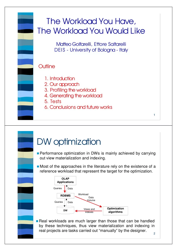
DW optimization

Performance optimization in DWs is mainly achieved by carrying

• ut view materialization and indexing.

Most of the approaches in the literature rely on the existence of a

reference workload that represent the target for the optimization.

DW

RDBMS OLAP Applications Optimization algorithms

Queries Data Queries Data Workload Views and indexes Data Volume

Real workloads are much larger than those that can be handled

by these techniques, thus view materialization and indexing in real projects are tasks carried out “manually” by the designer.

3

The reference framework

DW

RDBMS OLAP Applications Profiling & Clustering Optimization algorithms

Queries Data Queries Data Log Workload Profile Views and indexes Data volume

The optimization process can be driven by

• that shows the best choices to the designer.

The gap between academic approaches and real systems could

be filled by techniques capable of determining the workload characteristics while maintaining a reduced computational complexity.

4

Basics

Some of the indicators are based on the concept of cardinality of

the aggregation pattern associated to a given view .

The cardinality of an aggregation pattern can be estimated using

the Cardenas’ formula where |0| is the cardinality of the base fact table, while ||Max is the maximum number of tuples feasible for the pattern

( )

| | , | | ) (

max

• Φ

=

The

• f a given pattern representing a query

(or equivalently view) is computed as: | | ) ( 1 ) (

• −

=

() ranges in [0..1[

unaggregated pattern (i.e. the pattern of the base fact table)

0.9999 completely aggregated pattern

5

The average aggregation level

∑

=

=

• 1

) ( 1

The aggregation level () of the full workload is then

computed as: where is the number of queries in the workload.

• Workloads with high values of will be efficiently optimized

using views

Views determine a strong reduction of the number of tuples to be read Their limited size allows a higher number of views to be materialized

6

Skewness I

Workloads with similar values of can behave differently { } { } Materializing a single view to answer both the queries in the

workload is much more useful for 1 than for 2 since in the first case the is very close to the queries and still coarse.

• W

W1

1

W W2

2

Given two queries with patterns P1 and P2, their ancestor ancestor is the most aggregated pattern P1 P2 on wich both queries can be answered.

7

Skewness I

Workloads with similar values of can behave differently { } { } Materializing a single view to answer both the queries in the

workload is much more useful for 1 than for 2 since in the first case the is very close to the queries and still coarse.

• The difference is captured by the distance between two patterns

that is calculated as: Dist(Pi, Pj) = Agg(Pi) + Agg(Pj) - 2 Agg(Pi ⊕ Pj) W W1

1

W W2

2

8

Skewness II

The average skewness () of the full workload is calculated as: Workload with low values for will be efficiently optimized

using materialized views since the similarity of the query patterns makes it possible to materialize few views to optimize several queries

( )∑ ∑

− = + =

− ⋅ =

1 1 1

) , ( 1 2

9

Selectivity Indicators I

Profiling of selectivity is harder since the evaluation of the indicators

must be based on the values of those of the aggregation ones.

The main indicator is the average selectivity (): Workload with low values for will require stronger use of

indexes.

is not sufficient to characterize the impact of indexing with

respect to materialization since it depends on and the statements are formulated.

( ) ∑

=

=

• 1

1

10

Selectivity Indicators II

• On aggregated or un-aggregated patterns ?

≈ 0 selectivity is equally distributed < 0 selectivity is stronger for queries on aggregated patterns > 0 selectivity is stronger for queries on un-aggregated

patterns

( ) ( ) Very selective queries on fine patterns Low selective queries

• n coarse patterns

is the coefficient of the least-square error line

11

Selectivity Indicators III

• How many predicates are applied in the average on a query?

Where is the number of constrained tables on query Given a selectivity value , workload with higher values of

will require a higher number of indexes to apply all the conditions profitably.

∑

=

=

• 1

1

12

Workload Generation

An algorithm for generating a GPSJ workload has been devised

Testing: easily create large workloads Benchmarking: create workloads with specific characteristics

Generation of Patterns Generation of Selection criteria P, , opt,|W | , opt, |W | Unable to match opt

• W

Given a desired profile opt:

• a taboo-search

approach, navigating the multidimensional lattice, have been adopted.

• selectivity

is added exploiting the relationships between the generated patterns and the profile.

( ) ( ) (1) (2) (3)(4) (5) (1) (2) (3) (4) (5) () atan()

13

Test 20 I

Tests, carried out generating workloads based on the TPC-H/R

benchmark, are aimed at evaluating the correlation between

• ptimization and profile.

??? >36158 0.668 0.352 30 WKL6 14 99 0.316 0.884 30 WKL5 2 868 0.751 0.384 20 WKL4 15 596 0.810 0.790 20 WKL3 2 124 0.327 0.186 20 WKL2 15 97 0.348 0.835 20 WKL1

• WKL2

WKL1 WKL3 WKL4

2 4 6 8 10 12

1.1 1.4 1.7 2 2.3 2.6 2.9

Disk space constraint (GB) Millions of disk pg.

5 10 15 20 1.1 1.4 1.7 2 2.3 2.6 2.9 Disk space constraint (GB)

• N. of mat. views

14

Test 20 II

The second test measures the effect of selectivity

29.9 % 48.8 % 52.6 % 4.9 % 7.8 % 2.1 %

• 67% - 33%

22.0 % 2 0.5 0.751 0.384 WKL4c 68% - 32% 28.1 % 2 0.25 0.751 0.384 WKL4b 77% - 23% 27.3 % 2 0.04 0.751 0.384 WKL4a 84% - 16% 88.9 % 2 0.5 0.348 0.835 WKL1c 84% - 16% 88.2 % 2 0.25 0.348 0.835 WKL1b 59% - 41% 96.7 % 2 0.04 0.348 0.835 WKL1a

• 62.2 %

62.9 % 0.26 % 14.7 %

• 18.0 %

2.8 0.1 0.29 0.607 0.542 WKL7d 25.9 % 1.2 0.0 0.3 0.607 0.542 WKL7c 54.3 % 1.1

• 0.8

0.366 0.607 0.542 WKL7b 61.8 % 1 0.8 0.349 0.607 0.542 WKL7a

15

Test 200

Large workloads must be pre-reduced in order to apply optimization

algorithms.

Pre-optimization (clustering) progressively affects the workload

profile

! ! "#! "#! "$! "$! % % %&! %&! "%& "%& $ $ ''! ''! "! "! #! #! %($ %($ %#! %#! " " ( ( ' ! ' ! #! #! %! %! %(# %(# %'&! %'&! &'&& &'&& $ $ )*+# )*+# (&! (&! &! &! '(! '(! ( ( %$'! %$'! # # $ $ ((! ((! &(! &(! ( ! ( ! ""# ""# %((! %((! &## &## ( ( ((! ((! &(! &(! ($! ($! "( "( %(&! %(&! ( ( $ $ )*+% )*+%

• $

$ $$ $$ $'( $'( $$# $$# $# ( $# ( )*+# )*+# % % $$ $$ $ $ $'"% $'"% $"'% $"'% )*+% )*+%

• Indexing oriented

Materialization oriented 16

Conclusions

The profile has proved to be representative of the workload

characteristics.

The workload generation algorithm is the first attempt in the

database field to define large and ad-hoc workloads for benchmarking.

Transforming qualitative information in quantitative ones by

means of functions that, based on the workload profile allow the execution cost to be estimated.

& Future works