
SLIDE 1
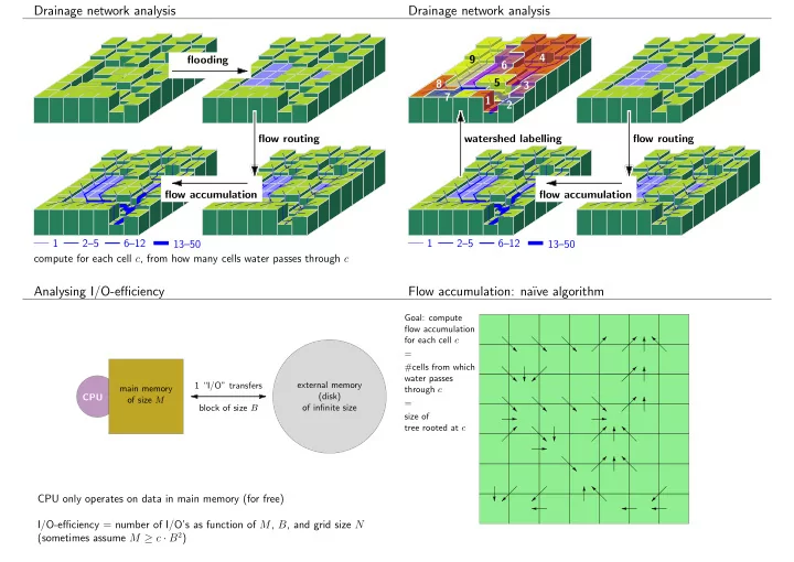
Drainage network analysis
1 2–5 6–12 13–50 flow routing compute for each cell c, from how many cells water passes through c flooding flow accumulation 1 2–5 6–12 13–50 1 2 4 6 8 7 3
Drainage network analysis
flow routing watershed labelling flow accumulation 9 5
Analysing I/O-efficiency
main memory
- f size M
external memory (disk)
- f infinite size