SLIDE 1 Draft
EE 8235: Lecture 21 1
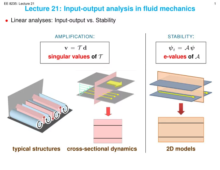
Lecture 21: Input-output analysis in fluid mechanics
- Linear analyses: Input-output vs. Stability
AMPLIFICATION:
v = T d singular values of T
STABILITY:
ψt = A ψ e-values of A
typical structures
typical structures cross-sectional dynamics 2D models
SLIDE 2 Draft
EE 8235: Lecture 21 2
Transition in Newtonian fluids
- LINEAR HYDRODYNAMIC STABILITY: unstable normal modes
⋆ successful in: Benard Convection, Taylor-Couette flow, etc. ⋆ fails in: wall-bounded shear flows (channels, pipes, boundary layers)
Inability to predict: Reynolds number for the onset of turbulence (Rec) Experimental onset of turbulence:
no sharp value for Rec
Inability to predict: flow structures observed at transition (except in carefully controlled experiments)
SLIDE 3 Draft
EE 8235: Lecture 21 3
LINEAR STABILITY: ⋆ For Re ≥ Rec ⇒
- exp. growing normal modes
corresponding e-functions (TS-waves)
- := exp. growing flow structures
✲
x
✂✂ ✍
z EXPERIMENTS: streaky boundary layers and turbulent spots
✲
x
✻
z
∞
✲
x
✻
z Matsubara & Alfredsson, J. Fluid Mech. ’01
SLIDE 4 Draft
EE 8235: Lecture 21 4
- FAILURE OF LINEAR HYDRODYNAMIC STABILITY
caused by high flow sensitivity ⋆ large transient responses ⋆ large noise amplification ⋆ small stability margins
TO COUNTER THIS SENSITIVITY:
must account for modeling imperfections TRANSITION ≈ STABILITY + RECEPTIVITY + ROBUSTNESS ← − ← − flow disturbances unmodeled dynamics
SLIDE 5 Draft
EE 8235: Lecture 21 5
Tools for quantifying sensitivity
- INPUT-OUTPUT ANALYSIS: spatio-temporal frequency responses
✲
d Free-stream turbulence Surface roughness Acoustic waves Linearized Dynamics
✲
Fluctuating velocity field
d1 d2 d3
d
amplification − − − − − − − − − − − → u v w
v
IMPLICATIONS FOR:
transition: insight into mechanisms control: control-oriented modeling
SLIDE 6 Draft
EE 8235: Lecture 21 6
Ensemble average energy density
Re = 2000
- Dominance of streamwise elongated structures
streamwise streaks!
SLIDE 7 Draft
EE 8235: Lecture 21 7
Influence of Re: streamwise-constant model
ψ2t
Re Acp Asq ψ1 ψ2
B3 B1 d1 d2 d3 u v w = Cu Cv Cw
ψ2
d2 B2
✲ ♥ ✲ (jωI − Aos)−1
Orr-Sommerfeld
s ✲ReAcp
coupling
✲ ♥ ✲ (jωI − Asq)−1
Squire
✲
ψ2 Cu
✲
u
✲
d1 B1
❄ ✲
d3 B3
✻ s ✲ Cv ✲
v
✲ Cw ✲
w ψ1 Jovanovi´ c & Bamieh, J. Fluid Mech. ’05
SLIDE 8 Draft
EE 8235: Lecture 21 8
Amplification mechanism in flows with high Re
- HIGHEST AMPLIFICATION: (d2, d3) → u
✲
d2 B2
✲ ♥ ✲(jωI − ∆−1∆2)−1
‘glorified diffusion’
✲
ψ1 ReAcp vortex tilting
✲ (jωI − ∆)−1
viscous dissipation
✲
ψ2 Cu
✲
u
✲
d3 B3
✻
☞ AMPLIFICATION MECHANISM: vortex tilting or lift-up wall-normal direction spanwise direction
SLIDE 9
Draft
EE 8235: Lecture 21 9
Turbulence without inertia
NEWTONIAN: inertial turbulence VISCOELASTIC: elastic turbulence Groisman & Steinberg, Nature ’00 NEWTONIAN: VISCOELASTIC: ☞ FLOW RESISTANCE: increased 20 times!
SLIDE 10
Draft
EE 8235: Lecture 21 10
Turbulence: good for mixing . . .
Groisman & Steinberg, Nature ’01
SLIDE 11
Draft
EE 8235: Lecture 21 11
. . . bad for processing
POLYMER MELT EMERGING FROM A CAPILLARY TUBE Kalika & Denn, J. Rheol. ’87 CURVILINEAR FLOWS: purely elastic instabilities Larson, Shaqfeh, Muller, J. Fluid Mech. ’90 RECTILINEAR FLOWS: no modal instabilities
SLIDE 12 Draft
EE 8235: Lecture 21 12
Oldroyd-B fluids
HOOKEAN SPRING: (Re/We) vt = − Re (v · ∇) v − ∇p + β ∆v + (1 − β) ∇ · τ + d 0 = ∇ · v τ t = − τ + ∇v + (∇v)T + We
- τ · ∇v + (∇v)T · τ − (v · ∇)τ
- VISCOSITY RATIO:
β := solvent viscosity total viscosity WEISSENBERG NUMBER: We := fluid relaxation time characteristic flow time REYNOLDS NUMBER: Re := inertial forces viscous forces
SLIDE 13 Draft
EE 8235: Lecture 21 13
Input-output analysis
✲
body forcing fluctuations Equations of motion
t ✲
velocity fluctuations
✛
Constitutive equations
t ✛
polymer stress fluctuations
✲
d1 d2 d3
d
amplification − − − − − − − − − − − → u v w
v
- INSIGHT INTO AMPLIFICATION MECHANISMS
importance of streamwise elongated structures Hoda, Jovanovi´ c, Kumar, J. Fluid Mech. ’08, ’09 Jovanovi´ c & Kumar, JNNFM ’11
SLIDE 14 Draft
EE 8235: Lecture 21 14
Inertialess channel flow: worst case amplification
- No single constitutive equation can describe the range of phenomena
⋆ important to quantify influence of modeling imperfections on dynamics We = 10, β = 0.5, Re = 0 G(kx, kz) = sup
ω σ2 max (T (kx, kz, ω)):
SLIDE 15
Draft
EE 8235: Lecture 21 15
We = 50, β = 0.5, Re = 0 G(kx, kz):
SLIDE 16 Draft
EE 8235: Lecture 21 16
We = 100, β = 0.5, Re = 0 G(kx, kz):
- Dominance of streamwise elongated structures
streamwise streaks!
SLIDE 17 Draft
EE 8235: Lecture 21 17
Amplification mechanism
- Highest amplification: (d2, d3) → u
INERTIALESS VISCOELASTIC:
✲
normal/spanwise forcing − 1 jωβ + 1 A−1
‘glorified diffusion’
✲ ✲We Acp2
polymer stretching
✲ − (1 − β)
jωβ + 1 ∆−1 viscous dissipation
✲
streamwise velocity INERTIAL NEWTONIAN:
✲
normal/spanwise forcing (jωI − Aos)−1 ‘glorified diffusion’
✲ ✲ ReAcp1
vortex tilting
✲
(jωI − ∆)−1 viscous dissipation
✲
streamwise velocity
SLIDE 18 Draft
EE 8235: Lecture 21 18
Inertialess lift-up mechanism
∆ ηt = −(1/β)∆η + We (1 − 1/β) Acp2 ϑ = −(1/β)∆η + We (1 − 1/β)
- ∂yz (U ′(y) τ22) + ∂zz (U ′(y) τ23)
SLIDE 19
Draft
EE 8235: Lecture 21 19
Spatial frequency responses
(d2, d3) amplification − − − − − − − − − − − → u INERTIAL NEWTONIAN: G(kz; Re) = Re2 f(kz) INERTIALESS VISCOELASTIC: G(kz; We, β) = We2 g(kz) (1 − β)2 vortex tilting: f(kz) polymer stretching: g(kz)
SLIDE 20 Draft
EE 8235: Lecture 21 20
Dominant flow patterns
☞ streamwise vortices and streaks Inertial Newtonian: Inertialess viscoelastic:
- CHANNEL CROSS-SECTION VIEW:
- color plots:
streamwise velocity contour lines: stream-function
SLIDE 21 Draft
EE 8235: Lecture 21 21
Flow sensitivity vs. nonlinearity
- Challenge: relative roles of flow sensitivity and nonlinearity
- Newtonian fluids: self-sustaining process for transition to turbulence
Waleffe, Phys. Fluids ’97
O(1/R) O(1/R) O(1)
Streaks Streak wave mode (3D) Streamwise self−interaction nonlinear U(y,z) instability of Rolls advection of mean shear