
SLIDE 1
Distributed Practice!
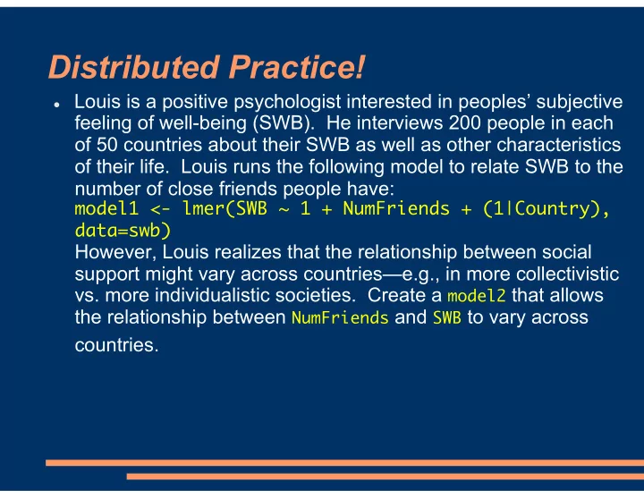
Louis is a positive psychologist interested in peoples’ subjective
feeling of well-being (SWB). He interviews 200 people in each
- f 50 countries about their SWB as well as other characteristics
- f their life. Louis runs the following model to relate SWB to the
number of close friends people have:
model1 <- lmer(SWB ~ 1 + NumFriends + (1|Country), data=swb)
However, Louis realizes that the relationship between social support might vary across countries—e.g., in more collectivistic
- vs. more individualistic societies. Create a model2 that allows