Discrete space (lattice) arises naturally in solids (crystals) Using - PowerPoint PPT Presentation

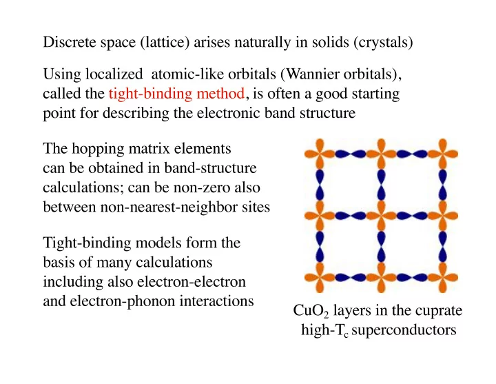
Discrete space (lattice) arises naturally in solids (crystals) Using localized atomic-like orbitals (Wannier orbitals), called the tight-binding method, is often a good starting point for describing the electronic band structure The hopping matrix elements can be obtained in band-structure calculations; can be non-zero also between non-nearest-neighbor sites Tight-binding models form the basis of many calculations including also electron-electron and electron-phonon interactions CuO 2 layers in the cuprate high-T c superconductors

Lanczos diagonalization Real-space discretized Hamiltonian is large in terms of N*N Ø but number of non-zero elements is ~N, not N 2 Ø sparse matrix eigenvalue problem Ø can use special methods for extremal eigenvalues/states The Lanczos method is a Krylov space method Ø space spanned by vectors Idea: operate on expansion in energy eigenstates For large m state with largest |E k | dominates the sum Ø Acting multiple times with H projects out extremal state Get ground state by acting with Ø we will assume that a suitable constant has been included Idea is to diagonalize H in space of all Ø can give low-lying states for small m (e.g., 100-500)

Lanczos basis states Particular orthogonal basis of states Ø leads to a tridiagonal Hamiltonian matrix Ø starts from arbitrary state First, orhogonal but not normalized basis Chose constant such that the two states are orthogonal Next state; make it orthogonal to the two previous ones:

One can show that these states are orthogonal to all previous ones Hamiltonian acting on a state This corresponds to a tri-diagonal matrix, non-zero elements are Normalized states

Algorithm for constructing the basis and the Hamiltonian For the Hamiltonian, we need only the factors where To obtain a new state we need the previous two: We have to store two states and the one we are working on. (numbers f n (j), j=1,...,N stored) We do not have to store H; act with it “ on the fly ” (V includes diag part of K) Need change in element index as particle “ hops ” between neigbors

1D test: Open chain (hard-wall box), x=[-1,1] (L=2), V=0 Calculated energies as a function of Lanczos basis size M 10 165.47488 1116.18787 3077.75501 N=200 20 36.464497 268.910471 744.48445 30 15.339143 155.724962 332.96633 40 11.382975 86.779071 196.57548 50 9.172055 47.562526 146.64266 Very poor 60 7.387181 27.980120 86.13795 70 4.460574 16.659015 62.67232 convergence 80 2.961753 14.353851 55.00397 90 2.219407 13.280460 41.92692 100 1.696802 12.229263 27.56645 Almost the full 110 1.416573 11.376356 22.04370 Hilbert space has 120 1.320332 10.941645 20.09118 130 1.288321 10.732066 19.15900 to be included to 140 1.276327 10.613516 18.51138 get good energies 150 1.262146 10.191426 14.60174 160 1.234164 6.045649 11.09876 170 1.224724 5.160069 11.01756 Deviations at M=200 180 1.222428 4.974962 11.00148 190 1.221635 4.905657 10.99395 reflect discretization 200 1.221430 4.885423 10.99108 error (negative) Exact 1.233701 4.934802 11.10330

Convergence of the ground state wave function Lanczos method is not suitable for this type of calculation in 1D Ø The basis must be of same size as the original one

2D test: Open box (=hard-wall), x,y=[-1,1], V=0 Energy as a function of Lanczos basis size M 20 146.53700 731.057995 1807.662851 N=200*200 40 36.89144 197.708305 466.352106 60 19.78221 88.403669 216.571047 80 14.33864 52.011927 120.846453 100 11.36276 33.130912 78.125621 Convergence 120 9.836334 25.714048 59.319176 140 9.093991 21.690312 43.007222 after on the 160 8.460393 17.444110 31.878198 order of 180 7.719381 13.667132 26.425252 iterations 200 6.494491 10.987755 22.538540 240 5.310526 9.837896 18.969252 280 3.925524 7.766020 11.142274 The method 320 2.815453 6.526244 10.305297 works better 360 2.482839 6.177734 9.963101 400 2.447032 6.119496 9.841073 in 2D 440 2.443210 6.108594 9.789598 480 2.442875 6.106960 9.772831 Exact 2.467401 6.168503 9.869604

The components (i.e., individual basis states) of the initial state must be propagated by the Hamiltonian through the whole system in order for an extended wave function to be representable in the Lanczos basis Regions covered after successive operations with H ( “ generations ” ) on a single basis state in 1D and 2D Covered fraction scales as the number of generations M in any D Ø The Lanczos scheme is advantageous in 2D and 3D