Differential geometry of sampled smooth surfaces: principal frames, - - PowerPoint PPT Presentation

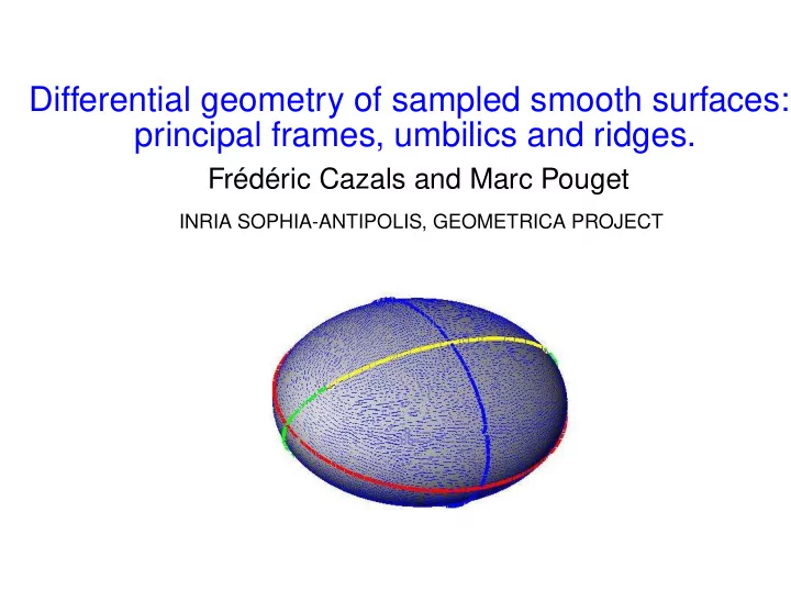
Differential geometry of sampled smooth surfaces: principal frames, umbilics and ridges.

Frédéric Cazals and Marc Pouget

INRIA SOPHIA-ANTIPOLIS, GEOMETRICA PROJECT

• I. Estimating Differential Quantities Using

Polynomial Fitting of Osculating Jets

• Symp. on Geometry Processing 2003.
• II. Classification of umbilics and ridges

Smooth surfaces, umbilics, lines of curvatures, foliations, ridges and the medial axis: a concise overview. Research report INRIA RR-5138.

• III. Algorithm for umbilics and ridges detec-

tion

Ridges and umbilics of a sampled smooth surface: a complete picture gearing toward topological coherence. Submitted.

Problem addressed

Input:

• S is a smooth surface embedded in R3.
• A triangulation or a point cloud sampled over S is provided.

Output:

• Estimate local differential properties of S: normal, curvatures, higher
• rder...
• Convergence results.

Contributions

• Method: polynomial fitting of arbitrary degree.
• Convergence analysis for interpolation and least square approxima-

tion.

• Error analysis of two stages methods.
• Experimental study.

Height functions and jets

y x x’ y’

Height function = jet + h.o.t: f(x,y) = JB,n(x,y)+O(||(x,y)||n+1)

JB,n(x,y) = B00 +B10x+B01y+B20x2 +B11xy+B02y2 +···+B0nyn.

JB,n, the Taylor expansion of f called the osculating n-jet, involves Nn =

1+2+···+(n+1) = (n+1)(n+2)/2 coefficients.

Differential Quantities

Unit normal vector nS = (−B10,−B01,1)t/

• 1+B2

10 +B2 01.

Second order info using the Weingarten map . . . {B10,B01,B20,B11,B02} Higher order info Retrieve the Monge form of the surface. z = 1 2(k1x2 +k2y2)+ 1 6(b0x3 +3b1x2y+3b2xy2 +b3y3) + 1 24(c0x4 +4c1x3y+6c2x2y2 +4c3xy3 +c4y4)+...

Fitting methods

Let pi(xi,yi, f(xi,yi)) be N sample points around the origin. Interpolation: find a n-jet JA,n: f(xi,yi) = JB,n(xi,yi)+O(||(xi,yi)||n+1) = JA,n(xi,yi), i = 1...N. Least-Square Approximation: find a n-jet JA,n minimizing:

N

∑

i=1

(JA,n(xi,yi)− f(xi,yi))2. Well poisedness of the problem and nearness to non-poised problems is measured by condition numbers.

Convergence issues

Surface: z = B00 +B10x+B01y+... Polynomial fi tting: z = A00 +A10x+A01y+...

O(h) S p pi x y z

The convergence is sought for a sequence of sample points function of the parameter h Wish: Ai j = Bi j +O(r(h))

Approximation results

Hypothesis: N points pi(xi,yi,zi), with xi = O(h),yi = O(h) Theorem [Interpolation or Approximation of degree n] Accuracy on coefficients of degree k of the Taylor expansion of f is O(hn−k+1): Ak− j,j = Bk− j,j +O(hn−k+1) ∀k = 0,...,n ∀ j = 0,...,k. Corollary

• unit normal coeffs estimated with accuracy O(hn),
• principal curvatures and directions estimated with accuracy O(hn−1)

Remarks

• A two step method (estimating normal first and curvatures later) is not

relevant.

• One has to fit a polynomial with all its coefficients, neglecting first
• rder coefficients leads to a loose of accuracy.
• Intuition:

higher the degree ⇐ ⇒ more degrees of freedom = ⇒ better fit.

• Error bounds instead of asymptotic convergence can be derived.
• Cf. P

.G. Ciarlet and P .-A. Raviart.

Algorithm

• 1. Collecting N samples
• Mesh case: ith rings
• PC case: local mesh, Power Diag. in the tangent plane, keep the

neighbors and discard weights.

X TX N

T

Natural neighbors

• and tangent-neighbors

Figure from J.D.Boissonnat and J.Flototto

Algorithm

• 2. Chose of the coordinate system
• Implicit plane fitting (PCA)
• the z-direction is the world coordinate axis with least angle w.r.t. the

normal of the fitted plane.

• 3. Fitting problem, degenerate cases —almost singular matrices
• Interpolation: choose samples differently
• Approximation: decrease degree, increase # pts
• 4. Retrieve Differential quantities
• Classical calculus.

Classical surfaces

(a)Elliptic paraboloid (16k points) (b)Surface of revolution (8k points)

Robustness on noisy model

.

• I. Estimating Differential Quantities Using

Polynomial Fitting of Osculating Jets

• II. Classification of umbilics and ridges
• 1. Introduction
• 2. Monge patch
• 3. Umbilics
• 4. Contact and ridges
• 5. Medial Axis
• III. Algorithm for umbilics and ridges detec-

tion

• 1. Introduction: umbilics and lines of curvature

• 1. Introduction: ridges and crest lines

• 2. Monge patch

The surface is locally given by a height function at the origin in the principal frame: z = 1 2(k1x2 +k2y2)+ 1 6(b0x3 +3b1x2y+3b2xy2 +b3y3) + 1 24(c0x4 +4c1x3y+6c2x2y2 +4c3xy3 +c4y4)+... In this Monge coordinate system, the Taylor expansion of the blue (max) curvature along the blue curvature line going through the origin has ex- pansion: k1(x) = k1 +b0x+ P

1

2(k1 −k2)x2 +... P

1 = 3b2 1 +(k1 −k2)(c0 −3k3 1).

Rk: switching the orientation of the principal directions reverts the sign of

• dd degree coefficients.

• 3. Umbilics: generic classifi cation

A curvature line is an integral curve of the principal direction field. Umbilics are singularities of these fields, they are classified by:

• the index, which is the number of turns of the principal field along a

circuit around the umbilic. It is ±1/2.

• the limiting principal directions, which are tangent directions to lines
• f curvature ending at the umbilic. There are 1 or 3 such directions.

Rk: the principal field is not orientable close to an umbilic

• 3. Umbilics: Lemon, Monstar and Star
• Lemon: index +1/2, 1 limiting principal direction.
• Monstar: index +1/2, 3 limiting principal directions.
• Star: index -1/2, 3 limiting principal directions.

Figures from Porteous, Geometric differentiation

• 4. Contact: defi nition

The surface S is parameterized by a Monge patch z(x,y). C is the sphere of center c(0,0,r) passing through the origin.

C S

c

z(x,y)

(x,y)

• Definition. 1 The contact function at the origin between the surface and

the sphere C is: g(x,y) = distance(z(x,y),c)2 −(radius of C)2 = x2(1−rk1)+y2(1−rk2)− r 3CM(x,y)+... Rk: g(x,y) = 0 ⇐ ⇒ (x,y,z(x,y)) ∈ C ∩S

• 4. Contact: singularities
• Definition. 2 Let f(x,y) be a smooth bivariate function. Function f has an

Ak or Dk singularity if, up to a diffeomorphism, it can be written as:

• Ak : f = ±x2 ±yk+1, k ≥ 0,

Dk : f = ±yx2 ±yk−1, k ≥ 4. (1) The singularity is further denoted A±

k or D± k if the product of the coefficients

• f the monomials is ±1.
• ✁

• ✁

• ✁

• ✁

Zero level sets of the Ak : f = x2 ±yk+1 singularities

• 5. Contact: A2

The sphere is a sphere of curvature of radius 1/k1 or 1/k2 Contact with the blue sphere Contact with the red sphere

• 4. Contact: A3 with the blue sphere

The blue sphere of curvature has radius 1/k1 and b0 = 0. Recall the expansion of k1 along the blue line: k1(x) = k1 +b0x+ P

1

2(k1 −k2)x2 +... P

1 = 3b2 1 +(k1 −k2)(c0 −3k3 1).

The contact point is called a ridge point:

• elliptic if P1 < 0 then this is a A+

3 singularity and the blue curvature is

maximal along its line;

• hyperbolic if P1 > 0 then this is a A−

3 singularity and the blue curvature

is minimal along its line.

• 4. Contact: A3 with the blue sphere

Blue elliptic ridge point Blue hyperbolic ridge point

• n the blue curve
• n the green curve

A+

3 contact

A−

3 contact

Maximum of k1 Minimum of k1

• 4. Contact: A4 blue

The blue sphere of curvature has radius 1/k1, b0 = 0 and P1 = 0. The blue curvature has an infection along the blue line. This is a ridge turning point and the ridge changes from elliptic to hyper- bolic.

• ✁✄✂

• 4. Contact: at umbilics

Umbilics are distinguished by the number of ridges passing through:

• Elliptic or 3-ridge umbilic.

k1 is minimal and k2 is maximal.

• Hyperbolic or 1-ridge umbilic.

There are curves passing through the umbilic on which k1 and k2 are constant. Note that at a ridge point, the line of curvature is tangent to the level set of the principal curvature.

unsymmetric elliptic umbilic Hyperbolic umbilic Symmetric elliptic umbilic

Ridges change color at umbilic and are hyperbolic

• 4. Contact: Elliptic umbilics

Symmetric elliptic umbilic Unsymmetric elliptic umbilic Figures from P . Giblin, 2 and 3 dimensional patterns of the face. Elliptic umbilics are stars. Dashed lines are level sets of the blue curvature, Thin lines are blue curvature lines, Thick lines are blue ridges.

• 4. Contact: Hyperbolic umbilics

Star Lemon monstar Figures from P . Giblin, 2 and 3 dimensional patterns of the face.

• 5. Medial Axis: Defi nition

Let S be a closed surface embedded in R3 The medial axis MA(S) consists of the points of the open set R3\S having two or more nearest points on S. The contact sphere must not intersect the surface then its contact points are A+

1 or A+ 3 singularities.

The MA is composed of several sheets, its boundary corresponds to some elliptic ridge point of the surface.

• 5. Medial Axis: Stratifi ed structure
• ✁✄✂
• ☎

• ✆

• ☎
• ☎
• ✂
• ☎

• ☎
• ✆

• ✆

• ☎
• ☎

• ✆

• ☎
• ☎

• 5. Medial Axis: missing elliptic ridge points

The center of the sphere of curvature of a ridge point can fail to be on the boundary of the MA in two cases:

• the surface is inside the sphere which cannot be maximal (e.g. min.
• f k2 > 0),
• the surface intersects the sphere away from the ridge point.

• I. Estimating Differential Quantities Using

Polynomial Fitting of Osculating Jets

• II. Classification of umbilics and ridges
• III. Algorithm for umbilics and ridges detec-

tion

• 1. Preliminaries
• 2. Umbilics
• 3. Orientation and ridges
• 4. Rough algorithm for ridges
• 5. Correct ridges at umbilics
• 6. Crest lines and filtered ridge points

• 1. Preliminaries:

Input of algorithm

S is a triangulated surface. Each vertex of S has a Monge patch, that is:

• the normal vector,
• the principal directions with an orientation,
• the coefficients of the Monge patch (up to 4th order).

Such a surface can be generated by:

• a smooth surface and analytical calculus,
• a triangulation and our jet fitting algorithm

Output of algorithm

• Detect ridge color and type.
• Find the right connection of ridges at umbilics and other crossings.

• 1. Preliminaries: Patches around vertices

Patch = topological disk neighborhood around a vertex It is a union of triangles:

• initialized with the 1-ring,
• then add the nearest incident triangle without changing the topology
• f the patch (priority queue).
• ✁
• ✂
• ✄
• ☎
• ✆

• 2. Umbilics
• 1. Define a patch around each

vertex,

• 2. collect

vertices minimizing (k1 −k2) on their patch,

• 3. compute the index on the

contour of the patch. Moreover, 3rd order Monge coefficients gives:

• the number and the directions of the limiting principal directions,
• the number of ridges crossing at the umbilic, hence the type elliptic or

hyperbolic of the umbilic.

• 3. Ridge point and Orientation of an edge

Sign of b0 on an oriented blue line crossing a blue ridge k1(x) = k1+b0x+ P

1

2(k1 −k2)x2+...

b>0 b>0 b<0 b<0 b=0 Ridge max of k1

Warning: b0 is not defined globally.

• Observation. 1 If the orientation of the principal directions along a path is

"correct" (prolonged by continuity) then a blue ridge crosses the path iff b0 changes sign: b0(p)b0(q) < 0.

• 3. Ridge point and Orientation of an edge

Detection of the crossing of a ridge (blue dotted line) on an edge near a lemon umbilic

• 3. Orientation of an edge
• Definition. 3 Orienting an edge with the acute rule is to choose maximal

principal vectors at the two vertices of an edge which make an acute angle. On a smooth surface S, we assume that an edge connecting two points of S defines a unique path on S.

• Definition. 4 The orientation of the principal directions of an edge is said

to be correct if the orientation by continuity along the path on the surface beginning from one point leads to the orientation of the second point.

• 4. Rough algorithm for ridges

Processing an edge [p,q]:

• orient the edge with the acute rule
• a blue ridge point detected if b0(p)b0(q) < 0,
• the position of the ridge point r is computed by linear interpolation:

r = (|b0(q)|p+|b0(p)|q)/(|b0(q)|+|b0(p)|)

• differential quantities at r are defined by the same interpolation. For

example P1(r) gives the type (elliptic or hyperbolic) of the ridge point r.

p q S r

• 4. Rough algorithm for ridges

Processing a triangle: there are 0,1,2 or 3 edges with a blue ridge point,

• 2 points: join them by a segment,
• 3 points: join them to the center of the triangle
• the type of a ridge segment is defined by either:

– the 4th order quantities P1 of the ridge points or, – the 3rd order quantities b0 at the vertices for the orientation of the blue direction toward the ridge segment.

Blue elliptic ridge

(Max of Kmax) Blue lines of curvature

V1 V2 V3 R1 R2 b0>0 b0>0 b0>0

• 4. Rough algorithm for ridges

Models of 40k points.

• 5. Correct ridges at umbilics
• Define patches around umbilics so that 1 or 3 ridge points are de-

tected on edges of the contour.

• Connect these ridge points to the umbilic.
• Observation. 2 If the topology of the ridges is generic and all edges not

in umbilic patches have a correct orientation, then the topology of ridges is recovered.

• 6. Crest lines and sharp ridge points

A crest line is a ridge line of maximum of max(|k1|,|k2|). Crest lines are a subset of elliptic ridges. One may see these lines as the visually most salient curves on a surface.

• 6. Crest lines and sharp ridge points

If the principal curvatures are constant on a surface (for example a plane

• r a cylinder) then all points are ridge points.

Sharp ridge point: one can avoid ridge points with a small variation of

curvature requiring P/(k1 −k2) to be greater than a threshold. k1(x) = k1 +b0x+ P

1

2(k1 −k2)x2 +...

• 6. Crest lines and sharp ridge points:

Mechanical model

All ridges Unfiltered crest lines Filtered crest lines

• 6. Crest lines and sharp ridge points:

Mechanical model

Bibliography

• N. Amenta and M. Bern DCG 1999

Surface reconstruction by Voronoi fi ltering.

• D. Meek and D. Walton CAGD 2000

On surface normal and Gaussian curvature approximations given data sampled from a smooth surface.

• D. Cohen-Steiner and J.M. Morvan ACM SoCG 2003

Restricted delaunay triangulations and normal cycle.

• V. Borrelli, F

. Cazals and J.M. Morvan CAGD 2003 On the angular defect of triangulations and the pointwise approximation of curvatures. P .G. Ciarlet and P .-A. Raviart General Lagrange and hermit interpolation in Rn with applications to the fi nite element

• method. In Arch. Rational Mesh. Engrg.

P . W. Hallinan, P . Giblin et al. 1999 Two-and Three-Dimensional Patterns of the Face.

• R. Morris 1996

The sub-parabolic lines of a surface, in Mathematics of Surfaces VI, IMA new series 58

• I. Porteous 2001

Geometric Differentiation, Cambridge University Press

• K. Watanabe and A.G. Belyaev, Eurographics’01

Detection of salient curvature features on polygonal surfaces.

• X. Pennec, N. Ayache, and J.-P

. Thirion 2000 Landmark-based registration using features identifi ed through differential geometry. In

• I. Bankman, editor, Handbook of Medical Imaging. Academic Press