Detection and Quantification of Urban Greenhouse Gas Emissions: - - PowerPoint PPT Presentation

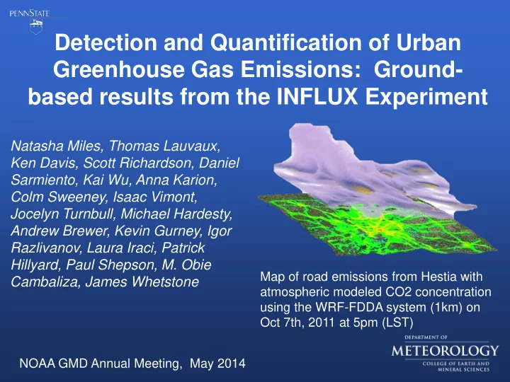
Detection and Quantification of Urban Greenhouse Gas Emissions: Ground- based results from the INFLUX Experiment

Map of road emissions from Hestia with atmospheric modeled CO2 concentration using the WRF-FDDA system (1km) on Oct 7th, 2011 at 5pm (LST)

Natasha Miles, Thomas Lauvaux, Ken Davis, Scott Richardson, Daniel Sarmiento, Kai Wu, Anna Karion, Colm Sweeney, Isaac Vimont, Jocelyn Turnbull, Michael Hardesty, Andrew Brewer, Kevin Gurney, Igor Razlivanov, Laura Iraci, Patrick Hillyard, Paul Shepson, M. Obie Cambaliza, James Whetstone

NOAA GMD Annual Meeting, May 2014

Goals of the Indianapolis Flux Experiment (INFLUX)

 Develop and assess methods of quantifying greenhouse gas emissions at the urban scale, using Indianapolis as a test bed.  In particular:

• Determine whole-city emissions of CO2 and CH4
• Measure emissions of CO2 and CH4 at 1 km2 spatial

resolution and weekly temporal resolution across the city

• Distinguish biogenic vs. anthropogenic sources of CO2
• Quantify and reduce uncertainty in urban emissions

estimates

Atmospheric measurement of GHG emissions

CO2, CO, CH4

 Compare to “Bottom-up” inventories using economic data and emissions factors  Atmospheric methods have the potential to provide independent emissions estimates  Measure GHG concentrations upwind and downwind of a source  Model atmospheric transport (wind, mixing depth)  Use an inversion to minimize the difference between modeled and

• bserved GHG concentrations

Steps

Vulcan and Hestia Emission Data Products

• Vulcan – hourly,

10km resolution for USA

• Hestia – hourly,

250 m resolution for Indianapolis, sector by sector

http://hestia.project.asu.edu/ Kevin Gurney Arizona State Univ

• Communications

towers ~100 m AGL

• Picarro, CRDS

sensors

• 12 measuring CO2, 5

with CH4, and 5 with CO

• NOAA automated

flask samplers

• NOAA LIDAR
• Eddy flux at 4 towers

INFLUX GROUND-BASED NETWORK

High resolution inversion modeling system

• Atmospheric model WRF-Chem: 9km/3km/1km (nested mode)
• Model physics

– Simple urban scheme within the NOAH Land Surface Model with the MYNN PBL scheme

• Coupled to Lagrangian Particle Dispersion Model (Uliasz, 1995)
• Bayesian Kalman matrix inversion
• Model assessment

– 4 eddy flux towers – NOAA HALO and HURDL Doppler Lidars – Aircraft data – Radiosonde campaign: 9-17 June

• Afternoon [CO2]

with 21-day smoothing

• Seasonal and

synoptic cycles are evident

• Site 03

(downtown): high [CO2]

• Site 01

(background): low [CO2]

Tower observations: [CO2] at INFLUX sites

2011 2012 2013

• Afternoon [CO2]

with 21-day smoothing

• Seasonal and

synoptic cycles are evident

• Site 03

(downtown): high [CO2]

• Site 01

(background): low [CO2]

Tower observations: [CO2] at INFLUX sites

• Site 09 measures

0.3 ppm larger than Site 01 (on average; changes with wind direction)

• Site 03 (downtown

site) measures larger [CO2] by 3 ppm

Spatial Structure of Urban CO2

Average [CO2] above background site

East of city Downtown

Afternoon daily values, 1 Jan – 1 April 2013

Eastern edge of city

• Spatial pattern of

emissions corrections (in %)

• Prior: Hestia 2002
• Tower observations

for Sept – Dec 2012

• Inversion decreased

emissions by up to 15% compared to Hestia 2002 in downtown region Lauvaux et al, in prep

Inversion results: spatial pattern of flux correction

• Prior: Hestia 2012
• Tower observations

for Sept – Dec 2012

• Corrections of -5 to

+5% rather than up to 15% change when using Hestia 2002/2011 as a prior Lauvaux et al, in prep

Inversion results: spatial pattern of flux correction

Inversion results

Sept 2012 Dec 2012 Hestia 2002: 1350 ktC Post using Hestia 2002: 1280 ktC Hestia 2011: 1345 ktC Post using Hestia 2011: 1274 ktC Hestia 2012: 1233 ktC Post using Hestia 2012: 1203 ktC

• Using 2012

tower data

• Inversion with

different priors

• Hestia 2002
• Hestia 2011
• Hestia 2012
• Inversion

converges to value towards 2012 values Lauvaux et al, in prep

How different is the emissions estimate using a different prior?

• ODIAC nightlight-based CO2 emissions product

(Tomohiro Odo) – Uses national petroleum and natural gas usage as total and distributes using nightlight data from satellite – Also incorporates power plant database – Available 1992 – 2012 worldwide

Hestia vs CDIAC Nightlight emissions product as prior

Odiac 2012: 1293 ktC Post using Odiac 2012: 1290 ktC Hestia 2012: 1233 ktC Post using Hestia 2012: 1203 ktC Posterior results are the within 10% of each other throughout the period, and 7% different overall Sept 2012 Dec 2012

Conclusions

• Tower observations detect a clear urban signal in CO2

(buried amid lots of synoptic “noise”). Differences vary greatly with weather conditions.

• Inversion converges to value towards Hestia 2012,

whichever version of prior estimate is used For more information, see http://influx.psu.edu